Viewing NEXRAD Level II Data¶

Overview¶

Within this notebook, we will cover:

How to access NEXRAD data from AWS
How to read this data into Py-ART
How to customize your plots and maps

Prerequisites¶

Concepts	Importance	Notes
Intro to Cartopy	Required	Projections and Features
Matplotlib Basics	Required	Basic plotting
Py-ART Basics	Required	IO/Visualization

Time to learn: 45 minutes

Imports¶

import pyart
import fsspec
from metpy.plots import USCOUNTIES
import matplotlib.pyplot as plt
import cartopy.crs as ccrs
import cartopy.feature as cfeature
import warnings
from datetime import datetime as dt
warnings.filterwarnings("ignore")

## You are using the Python ARM Radar Toolkit (Py-ART), an open source
## library for working with weather radar data. Py-ART is partly
## supported by the U.S. Department of Energy as part of the Atmospheric
## Radiation Measurement (ARM) Climate Research Facility, an Office of
## Science user facility.
##
## If you use this software to prepare a publication, please cite:
##
##     JJ Helmus and SM Collis, JORS 2016, doi: 10.5334/jors.119

<frozen importlib._bootstrap>:283: DeprecationWarning: the load_module() method is deprecated and slated for removal in Python 3.12; use exec_module() instead

ERROR 1: PROJ: proj_create_from_database: Open of /knight/anaconda_aug22/envs/aug22_env/share/proj failed

How to Access NEXRAD Data from Amazon Web Services (AWS)¶

Let’s start first with NEXRAD Level 2 data, which is ground-based radar data collected by the National Oceanic and Atmospheric Administration (NOAA), as a part of the National Weather Service (NWS) observing network.

Level 2 Data¶

Level 2 data includes all of the fields in a single file - for example, a file may include:

Reflectivity
Velocity

Search for Radar Data¶

We will access data from the noaa-nexrad-level2 bucket, with the data organized as:

s3://noaa-nexrad-level2/year/month/date/radarsite/{radarsite}{year}{month}{date}_{hour}{minute}{second}_V06

We can use fsspec, a tool to work with filesystems in Python, to search through the bucket to find our files!

We start first by setting up our AWS S3 filesystem

fs = fsspec.filesystem("s3", anon=True)

Once we set up our filesystem, we can list files from the site and date/time of our choice.

Select the date

datTime = dt(2023,3,31,23)
year = dt.strftime(datTime,format="%Y")
month = dt.strftime(datTime,format="%m")
day = dt.strftime(datTime,format="%d")
hour = dt.strftime(datTime,format="%H")

Specify the radar site

site = 'KLZK'

Specify latitude and longitude bounds for the resulting maps.

lonW = -95
lonE = -91
latS = 33
latN = 37

Construct the URL pointing to the radar file directory

url = f's3://noaa-nexrad-level2/{year}/{month}/{day}/{site}/{site}{year}{month}{day}_{hour}*V06'

url

's3://noaa-nexrad-level2/2023/03/31/KLZK/KLZK20230331_23*V06'

files = sorted(fs.glob(url))
files

['noaa-nexrad-level2/2023/03/31/KLZK/KLZK20230331_230250_V06',
 'noaa-nexrad-level2/2023/03/31/KLZK/KLZK20230331_230800_V06',
 'noaa-nexrad-level2/2023/03/31/KLZK/KLZK20230331_231309_V06',
 'noaa-nexrad-level2/2023/03/31/KLZK/KLZK20230331_231805_V06',
 'noaa-nexrad-level2/2023/03/31/KLZK/KLZK20230331_232247_V06',
 'noaa-nexrad-level2/2023/03/31/KLZK/KLZK20230331_232731_V06',
 'noaa-nexrad-level2/2023/03/31/KLZK/KLZK20230331_233216_V06',
 'noaa-nexrad-level2/2023/03/31/KLZK/KLZK20230331_233729_V06',
 'noaa-nexrad-level2/2023/03/31/KLZK/KLZK20230331_234227_V06',
 'noaa-nexrad-level2/2023/03/31/KLZK/KLZK20230331_234738_V06',
 'noaa-nexrad-level2/2023/03/31/KLZK/KLZK20230331_235304_V06',
 'noaa-nexrad-level2/2023/03/31/KLZK/KLZK20230331_235801_V06']

We now have a list of files we can read in!

Read the Data into PyART¶

When reading into PyART, we can use the pyart.io.read_nexrad_archive or pyart.io.read module to read in our data.

Read in the first radar file in the group.

radar = pyart.io.read_nexrad_archive(f's3://{files[0]}')

Notice how for the NEXRAD Level 2 data, we have several fields available

list(radar.fields)

['velocity',
 'differential_phase',
 'reflectivity',
 'differential_reflectivity',
 'clutter_filter_power_removed',
 'spectrum_width',
 'cross_correlation_ratio']

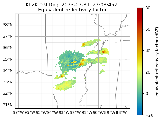
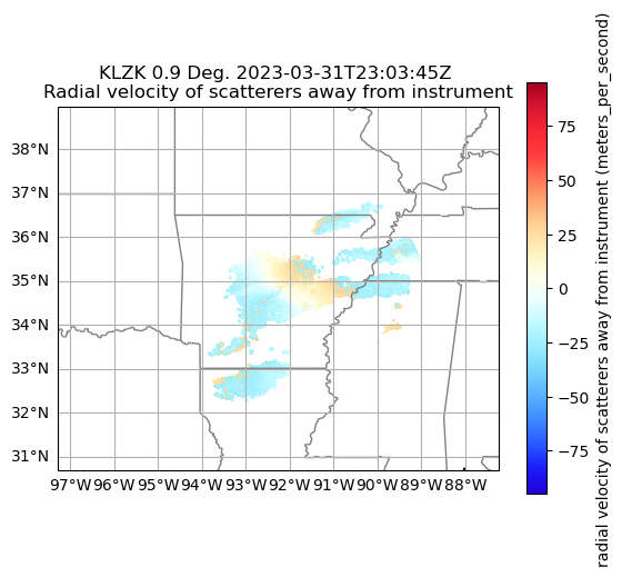
Plot a quick-look of the dataset¶

Let’s get a quick look of the reflectivity and velocity fields

display = pyart.graph.RadarMapDisplay(radar)

What options does plot_ppi_map give us?

display.plot_ppi_map?

The default resolution for the cartographic features is the coarsest (110m). Let’s crank it up to the finest resolution (‘10m’).

res = '10m'

display.plot_ppi_map('reflectivity',
                     sweep=3,
                     vmin=-20,
                     vmax=80,
                     projection=ccrs.PlateCarree(),
                     resolution=res
                    )

display.plot_ppi_map('velocity',
                     sweep=3,
                     projection=ccrs.PlateCarree(),
                     resolution=res
                    )

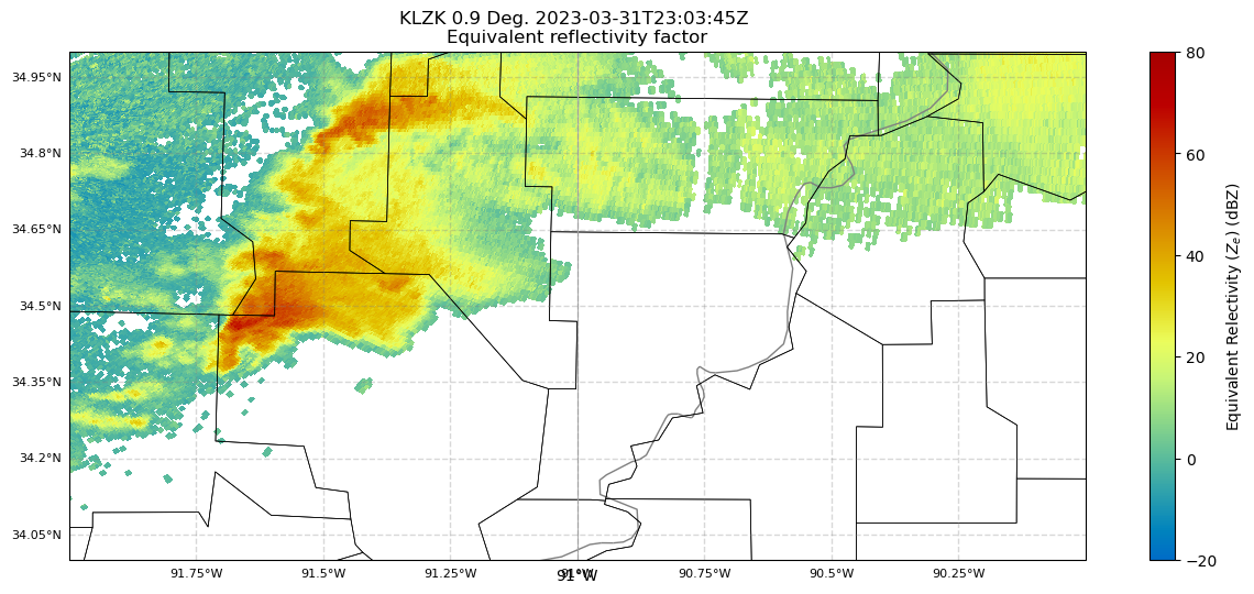
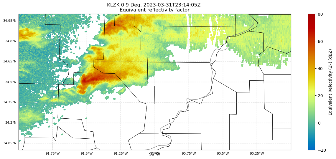
Create a single figure of reflectivity, zoomed into the main storm. Add counties and other enhancements.¶

lonW = -92
lonE = -90
latS = 34
latN = 35

# Create our figure
fig = plt.figure(figsize=[15, 6])

# Setup our first axis with reflectivity
ax1 = plt.subplot(111, projection=ccrs.PlateCarree())
display = pyart.graph.RadarMapDisplay(radar)
ref_map = display.plot_ppi_map('reflectivity',sweep=3, vmin=-20, vmax=80, ax=ax1, colorbar_label='Equivalent Relectivity ($Z_{e}$) (dBZ)', resolution=res)

ax1.set_extent ([lonW, lonE, latS, latN])

# Add gridlines
gl = ax1.gridlines(crs=ccrs.PlateCarree(), draw_labels=True, linewidth=1, color='gray', alpha=0.3, linestyle='--')

# Make sure labels are only plotted on the left and bottom
gl.xlabels_top = False
gl.ylabels_right = False

# Specify the fontsize of our gridline labels
gl.xlabel_style = {'fontsize':8}
gl.ylabel_style = {'fontsize':8}

# Add counties
ax1.add_feature(USCOUNTIES, linewidth=0.5);

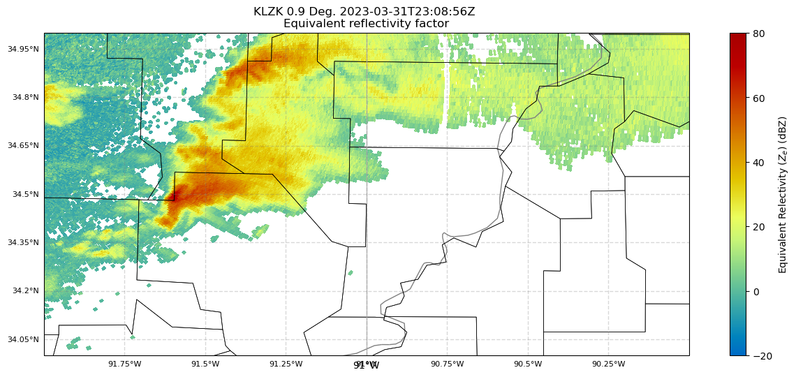
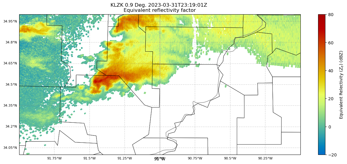
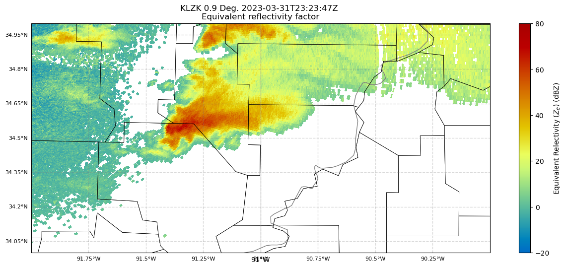
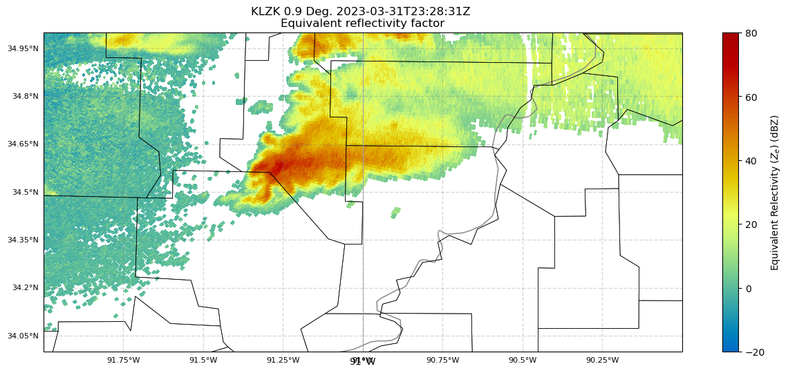
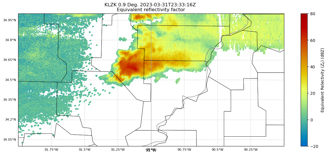
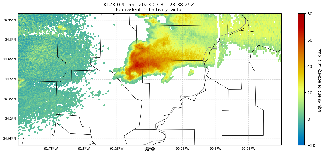
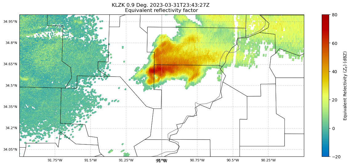
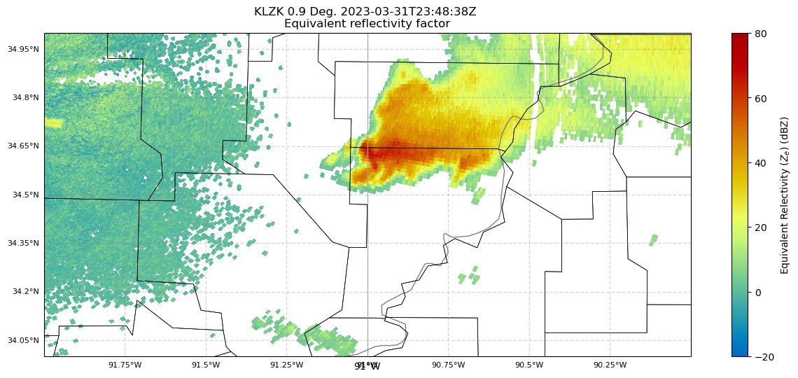
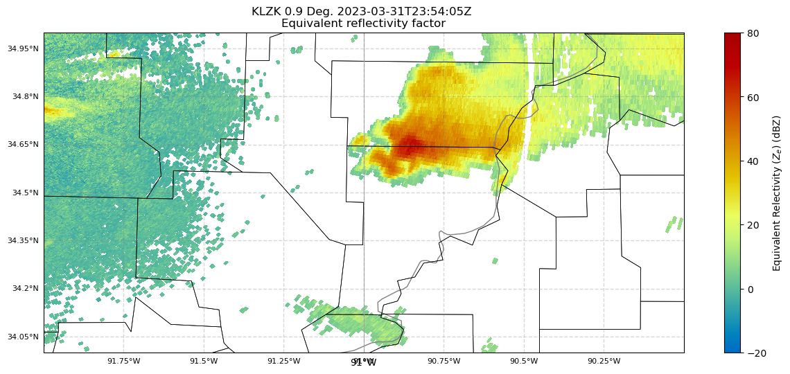
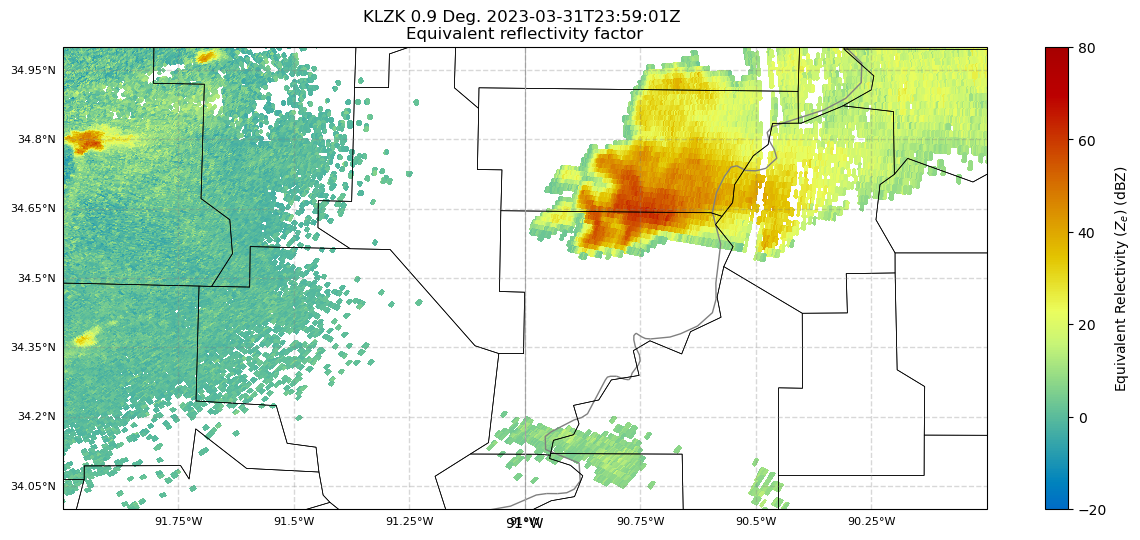
Next, let’s create a function that does the same as the previous cell, so we can loop over all the radar files of the specified hour.

def plot_radar_refl (idx, site):
    radar = pyart.io.read_nexrad_archive(f's3://{files[idx]}')    
    # Create our figure
    fig = plt.figure(figsize=[15, 6])

    # Set up our axes
    ax1 = plt.subplot(111, projection=ccrs.PlateCarree())
    display = pyart.graph.RadarMapDisplay(radar)
    ref_map = display.plot_ppi_map('reflectivity',sweep=3, vmin=-20, vmax=80, ax=ax1, colorbar_label='Equivalent Relectivity ($Z_{e}$) (dBZ)', resolution=res)

    ax1.set_extent ([lonW, lonE, latS, latN])

# Add gridlines
    gl = ax1.gridlines(crs=ccrs.PlateCarree(), draw_labels=True, linewidth=1, color='gray', alpha=0.3, linestyle='--')

# Make sure labels are only plotted on the left and bottom
    gl.xlabels_top = False
    gl.ylabels_right = False

# Specify the fontsize of our gridline labels
    gl.xlabel_style = {'fontsize':8}
    gl.ylabel_style = {'fontsize':8}

# Add counties
    ax1.add_feature(USCOUNTIES, linewidth=0.5)

# Save the figure.
    fNum = str(idx).zfill(2)
    figTitle = f'{site}_refl_{fNum}.png'
    fig.savefig(figTitle)

Loop over the files. Save each image.

for n, name in enumerate(files):
    print (n, name, site)
    plot_radar_refl(n, site)    

0 noaa-nexrad-level2/2023/03/31/KLZK/KLZK20230331_230250_V06 KLZK

1 noaa-nexrad-level2/2023/03/31/KLZK/KLZK20230331_230800_V06 KLZK

2 noaa-nexrad-level2/2023/03/31/KLZK/KLZK20230331_231309_V06 KLZK

3 noaa-nexrad-level2/2023/03/31/KLZK/KLZK20230331_231805_V06 KLZK

4 noaa-nexrad-level2/2023/03/31/KLZK/KLZK20230331_232247_V06 KLZK

5 noaa-nexrad-level2/2023/03/31/KLZK/KLZK20230331_232731_V06 KLZK

6 noaa-nexrad-level2/2023/03/31/KLZK/KLZK20230331_233216_V06 KLZK

7 noaa-nexrad-level2/2023/03/31/KLZK/KLZK20230331_233729_V06 KLZK

8 noaa-nexrad-level2/2023/03/31/KLZK/KLZK20230331_234227_V06 KLZK

9 noaa-nexrad-level2/2023/03/31/KLZK/KLZK20230331_234738_V06 KLZK

10 noaa-nexrad-level2/2023/03/31/KLZK/KLZK20230331_235304_V06 KLZK

11 noaa-nexrad-level2/2023/03/31/KLZK/KLZK20230331_235801_V06 KLZK

Summary¶

Within this example, we walked through how to use PyART to read in and plot NEXRAD Level 2 data for a location and hour of your choice.

Things to try¶

The above example is for reflectivity. Try additional radar products, such as velocity; also try different sweeps.

What’s next?¶

We will develop code to animate the sequence.

ATM350 Spring 2023

Viewing NEXRAD Level II Data

Contents