04_GriddedDiagnostics_Frontogenesis_CFSR: Compute derived quantities using MetPy
Contents
04_GriddedDiagnostics_Frontogenesis_CFSR: Compute derived quantities using MetPy
In this notebook, we’ll cover the following:
Select a date and access various CFSR Datasets
Subset the desired Datasets along their dimensions
Calculate and visualize frontogenesis.
Smooth the diagnostic field.
0) Preliminaries 
import xarray as xr
import pandas as pd
import numpy as np
from datetime import datetime as dt
from metpy.units import units
import metpy.calc as mpcalc
import cartopy.crs as ccrs
import cartopy.feature as cfeature
import matplotlib.pyplot as plt
ERROR 1: PROJ: proj_create_from_database: Open of /knight/anaconda_aug22/envs/aug22_env/share/proj failed
1) Specify a starting and ending date/time, and access several CFSR Datasets
startYear = 2007
startMonth = 2
startDay = 14
startHour = 12
startMinute = 0
startDateTime = dt(startYear,startMonth,startDay, startHour, startMinute)

endYear = 2007
endMonth = 2
endDay = 14
endHour = 12
endMinute = 0
endDateTime = dt(endYear,endMonth,endDay, endHour, endMinute)
Create Xarray Dataset objects
dsZ = xr.open_dataset ('/cfsr/data/%s/g.%s.0p5.anl.nc' % (startYear, startYear))
dsT = xr.open_dataset ('/cfsr/data/%s/t.%s.0p5.anl.nc' % (startYear, startYear))
dsU = xr.open_dataset ('/cfsr/data/%s/u.%s.0p5.anl.nc' % (startYear, startYear))
dsV = xr.open_dataset ('/cfsr/data/%s/v.%s.0p5.anl.nc' % (startYear, startYear))
dsW = xr.open_dataset ('/cfsr/data/%s/w.%s.0p5.anl.nc' % (startYear, startYear))
dsQ = xr.open_dataset ('/cfsr/data/%s/q.%s.0p5.anl.nc' % (startYear, startYear))
dsSLP = xr.open_dataset ('/cfsr/data/%s/pmsl.%s.0p5.anl.nc' % (startYear, startYear))
2) Specify a date/time range, and subset the desired Datasets along their dimensions.
Create a list of date and times based on what we specified for the initial and final times, using Pandas’ date_range function
dateList = pd.date_range(startDateTime, endDateTime,freq="6H")
dateList
DatetimeIndex(['2007-02-14 12:00:00'], dtype='datetime64[ns]', freq='6H')
# Areal extent
lonW = -90
lonE = -60
latS = 35
latN = 50
cLat, cLon = (latS + latN)/2, (lonW + lonE)/2
latRange = np.arange(latS,latN+.5,.5) # expand the data range a bit beyond the plot range
lonRange = np.arange(lonW,lonE+.5,.5) # Need to match longitude values to those of the coordinate variable
Specify the pressure level.
# Vertical level specificaton
pLevel = 850
levStr = f'{pLevel}'
We will display temperature and wind (and ultimately, temperature advection), so pick the relevant variables.
Now create objects for our desired DataArrays based on the coordinates we have subsetted.
# Data variable selection
T = dsT['t'].sel(time=dateList,lev=pLevel,lat=latRange,lon=lonRange)
U = dsU['u'].sel(time=dateList,lev=pLevel,lat=latRange,lon=lonRange)
V = dsV['v'].sel(time=dateList,lev=pLevel,lat=latRange,lon=lonRange)
Define our subsetted coordinate arrays of lat and lon. Pull them from any of the DataArrays. We’ll need to pass these into the contouring functions later on.
lats = T.lat
lons = T.lon
3) Calculate and visualize 2-dimensional frontogenesis.
In order to calculate many meteorologically-relevant quantities that depend on distances between gridpoints, we need horizontal distance between gridpoints in meters. MetPy can infer this from datasets such as our CFSR that are lat-lon based, but we need to explicitly assign a coordinate reference system first.
crsCFSR = {'grid_mapping_name': 'latitude_longitude', 'earth_radius': 6371229.0}
T = T.metpy.assign_crs(crsCFSR)
U = U.metpy.assign_crs(crsCFSR)
V = V.metpy.assign_crs(crsCFSR)
Unit conversions
UKts = U.metpy.convert_units('kts')
VKts = V.metpy.convert_units('kts')
constrainLat, constrainLon = (0.5, 4.0)
proj_map = ccrs.LambertConformal(central_longitude=cLon, central_latitude=cLat)
proj_data = ccrs.PlateCarree() # Our data is lat-lon; thus its native projection is Plate Carree.
res = '50m'
Let’s explore the frontogenesis diagnostic: https://unidata.github.io/MetPy/latest/api/generated/metpy.calc.frontogenesis.html
We first need to compute potential temperature. First, let’s attach units to our chosen pressure level, so that MetPy can calculate potential temperature accordingly.
#Attach units to pLevel for use in MetPy with new variable, P:
P = pLevel*units['hPa']
Now calculate potential temperature, and verify that it looks reasonable.
Thta = mpcalc.potential_temperature(P, T)
Thta
<xarray.DataArray (time: 1, lat: 31, lon: 61)>
<Quantity([[[277.17615 277.38568 278.74747 ... 289.74652 289.3275  289.3275 ]
  [276.44287 276.8619  277.8047  ... 289.43225 289.11798 289.22275]
  [276.54764 276.96664 277.38568 ... 289.74652 289.74652 289.85126]
  ...
  [263.03452 262.92975 263.03452 ... 279.79498 279.69022 279.37598]
  [262.406   262.09174 262.1965  ... 279.37598 279.48074 279.37598]
  [261.7775  261.56796 261.46323 ... 278.8522  279.0617  279.0617 ]]], 'kelvin')>
Coordinates:
  * time       (time) datetime64[ns] 2007-02-14T12:00:00
    lev        float32 850.0
  * lat        (lat) float32 35.0 35.5 36.0 36.5 37.0 ... 48.5 49.0 49.5 50.0
  * lon        (lon) float32 -90.0 -89.5 -89.0 -88.5 ... -61.5 -61.0 -60.5 -60.0
metpy_crs object Projection: latitude_longitudeNow calculate frontogenesis, and examine the output DataArray.
frnt = mpcalc.frontogenesis(Thta, U, V)
frnt
/knight/anaconda_aug22/envs/aug22_env/lib/python3.10/site-packages/pint/quantity.py:1313: RuntimeWarning: invalid value encountered in true_divide
  magnitude = magnitude_op(new_self._magnitude, other._magnitude)
<xarray.DataArray (time: 1, lat: 31, lon: 61)>
<Quantity([[[ 2.91151977e-10 -3.24387124e-10 -4.97951729e-10 ...  7.01957600e-10
    5.24068586e-10  3.35834349e-11]
  [-1.57035466e-11 -1.94215527e-10 -4.30818135e-10 ...  1.03789497e-10
    1.99768651e-11  1.71399062e-10]
  [ 2.17158493e-12  2.54716206e-13 -1.52830489e-10 ...  2.39948707e-10
    4.83354357e-10  3.64982783e-10]
  ...
  [ 1.39214392e-10  1.38258163e-10  3.32075745e-10 ...  1.15784003e-10
   -1.08017989e-11 -1.32146556e-10]
  [ 2.89824731e-10  1.25782966e-10  7.89610976e-11 ... -8.73358455e-11
   -5.08300616e-13 -5.73486450e-11]
  [ 3.27357863e-10  1.52502724e-10  1.07846382e-10 ... -4.50574964e-10
   -3.35488746e-10 -7.68334081e-11]]], 'kelvin / meter / second')>
Coordinates:
  * time       (time) datetime64[ns] 2007-02-14T12:00:00
    lev        float32 850.0
  * lat        (lat) float32 35.0 35.5 36.0 36.5 37.0 ... 48.5 49.0 49.5 50.0
  * lon        (lon) float32 -90.0 -89.5 -89.0 -88.5 ... -61.5 -61.0 -60.5 -60.0
metpy_crs object Projection: latitude_longitudeLet’s get a quick visualization, using Xarray’s built-in interface to Matplotlib.
frnt.plot(figsize=(15,10),cmap='coolwarm')
<matplotlib.collections.QuadMesh at 0x15306ac4dc90>
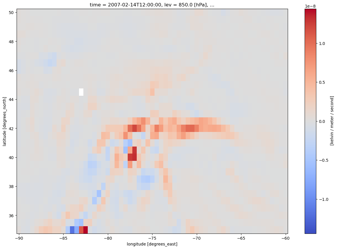
Note the white pixel near 44 N, 83 W. This likely is a NaN somehow resulting from the frontogenesis calculation.
The units are in degrees K (or C) per meter per second. Traditionally, we plot frontogenesis on more of a meso- or synoptic scale … degrees K/C per 100 km per 3 hours. Let’s simply multiply by the conversion factor.
# A conversion factor to get frontogensis units of K per 100 km per 3 h
convert_to_per_100km_3h = 1000*100*3600*3
frnt = frnt * convert_to_per_100km_3h
Check the range and scale of values.
frnt.min().values, frnt.max().values
(array(-12.74713155), array(15.57214382))
A scale of 1 (i.e., 1x10^0, AKA 1e0) looks appropriate.
scale = 1e0
Usually, we wish to avoid plotting the “zero” contour line for diagnostic quantities such as divergence, advection, and frontogenesis. Thus, create two lists of values … one for negative and one for positive.
frntInc = 3
negFrntContours = np.arange (-18, 0, frntInc)
posFrntContours = np.arange (3, 21, frntInc)
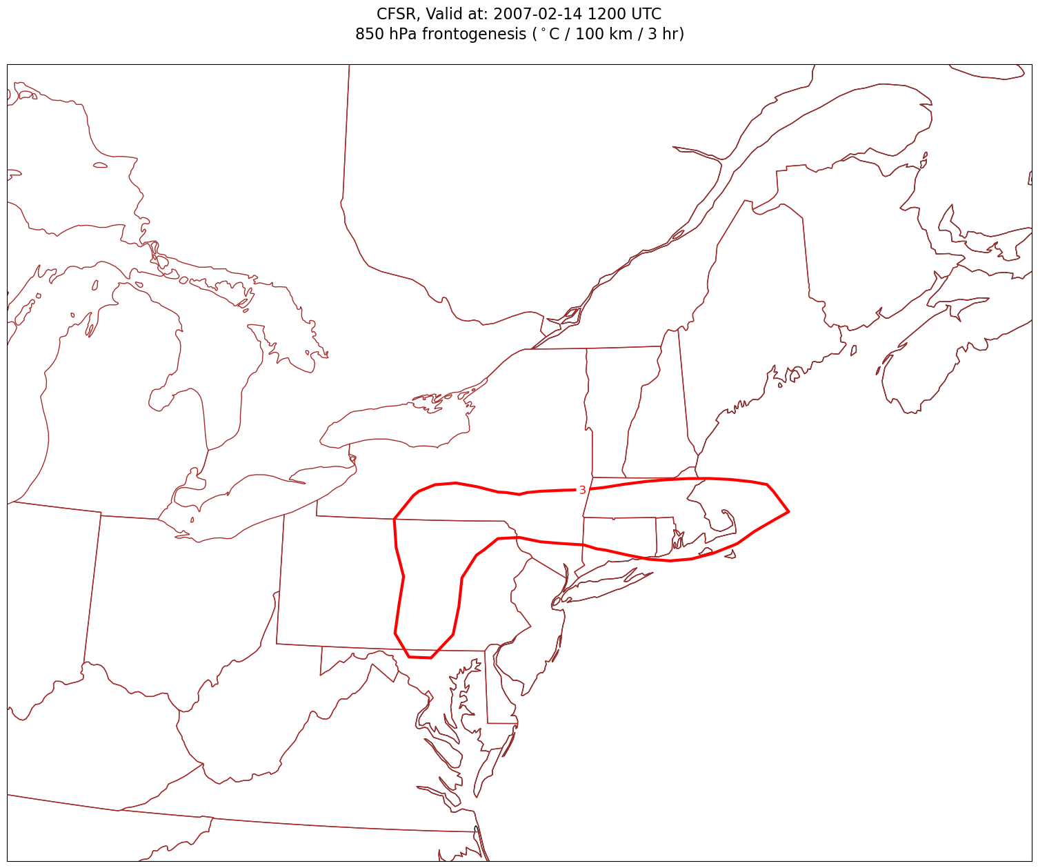
Now, let’s plot frontogenesis on the map.
for time in dateList:
    print("Processing", time)

    # Create the time strings, for the figure title as well as for the file name.
    timeStr = dt.strftime(time,format="%Y-%m-%d %H%M UTC")
    timeStrFile = dt.strftime(time,format="%Y%m%d%H")

    tl1 = str('CFSR, Valid at: '+ timeStr)
    tl2 = levStr + " hPa frontogenesis ($^\circ$C / 100 km / 3 hr)"

    title_line = (tl1 + '\n' + tl2 + '\n')

    fig = plt.figure(figsize=(21,15)) # Increase size to adjust for the constrained lats/lons
    ax = plt.subplot(1,1,1,projection=proj_map)
    ax.set_extent ([lonW+constrainLon,lonE-constrainLon,latS+constrainLat,latN-constrainLat])
    ax.add_feature(cfeature.COASTLINE.with_scale(res))
    ax.add_feature(cfeature.STATES.with_scale(res),edgecolor='brown')

    # Need to use Xarray's sel method here to specify the current time for any DataArray you are plotting.

    # 1a. Contour lines of warm (positive temperature) advection.
    # Don't forget to multiply by the scaling factor!
    cPosTAdv = ax.contour(lons, lats, frnt.sel(time=time)*scale, levels=posFrntContours, colors='red', linewidths=3, transform=proj_data)
    ax.clabel(cPosTAdv, inline=1, fontsize=12, fmt='%.0f')

    # 1b. Contour lines of cold (negative temperature) advection
    cNegTAdv = ax.contour(lons, lats, frnt.sel(time=time)*scale, levels=negFrntContours, colors='blue', linewidths=3, transform=proj_data)
    ax.clabel(cNegTAdv, inline=1, fontsize=12, fmt='%.0f')

    title = plt.title(title_line,fontsize=16)
    #Generate a string for the file name and save the graphic to your current directory.
    fileName = timeStrFile + '_CFSR_' + levStr + '_Frnt.png'
    fig.savefig(fileName)
Processing 2007-02-14 12:00:00
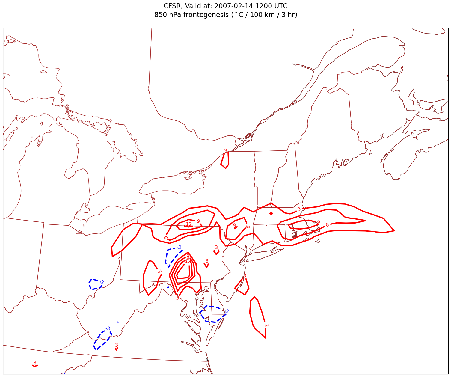
4. Smooth the diagnostic field.
Use MetPy’s implementation of a Gaussian smoother.
sigma = 10.0 # this depends on how noisy your data is, adjust as necessary
frntSmth = mpcalc.smooth_gaussian(frnt, sigma)
frntSmth.plot(figsize=(15,10),cmap='coolwarm')
<matplotlib.collections.QuadMesh at 0x153061cdf250>
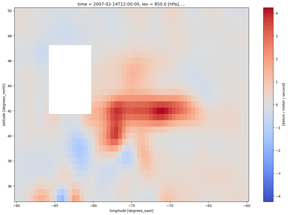
Plot the smoothed field.
for time in dateList:
    print("Processing", time)

    # Create the time strings, for the figure title as well as for the file name.
    timeStr = dt.strftime(time,format="%Y-%m-%d %H%M UTC")
    timeStrFile = dt.strftime(time,format="%Y%m%d%H")

    tl1 = str('CFSR, Valid at: '+ timeStr)
    tl2 = levStr + " hPa frontogenesis ($^\circ$C / 100 km / 3 hr)"

    title_line = (tl1 + '\n' + tl2 + '\n')

    fig = plt.figure(figsize=(21,15)) # Increase size to adjust for the constrained lats/lons
    ax = plt.subplot(1,1,1,projection=proj_map)
    ax.set_extent ([lonW+constrainLon,lonE-constrainLon,latS+constrainLat,latN-constrainLat])
    ax.add_feature(cfeature.COASTLINE.with_scale(res))
    ax.add_feature(cfeature.STATES.with_scale(res),edgecolor='brown')

    # Need to use Xarray's sel method here to specify the current time for any DataArray you are plotting.

    # 1a. Contour lines of warm (positive temperature) advection.
    # Don't forget to multiply by the scaling factor!
    cPosTAdv = ax.contour(lons, lats, frntSmth.sel(time=time)*scale, levels=posFrntContours, colors='red', linewidths=3, transform=proj_data)
    ax.clabel(cPosTAdv, inline=1, fontsize=12, fmt='%.0f')

    # 1b. Contour lines of cold (negative temperature) advection
    cNegTAdv = ax.contour(lons, lats, frntSmth.sel(time=time)*scale, levels=negFrntContours, colors='blue', linewidths=3, transform=proj_data)
    ax.clabel(cNegTAdv, inline=1, fontsize=12, fmt='%.0f')

    title = plt.title(title_line,fontsize=16)
    #Generate a string for the file name and save the graphic to your current directory.
    fileName = timeStrFile + '_CFSR_' + levStr + '_Frnt.png'
    fig.savefig(fileName)
Processing 2007-02-14 12:00:00
/knight/anaconda_aug22/envs/aug22_env/lib/python3.10/site-packages/cartopy/mpl/geoaxes.py:1614: UserWarning: No contour levels were found within the data range.
  result = super().contour(*args, **kwargs)