More NEXRAD Level II Visualization
Contents
More NEXRAD Level II Visualization
Overview
Within this notebook, we will cover:
Adding range rings to a PPI plot
Calculate and display a Velocity Azimuthal Display (VAD) profile
Prerequisites
Concepts |
Importance |
Notes |
|---|---|---|
Required |
Projections and Features |
|
Required |
Basic plotting |
|
Py-ART Basics |
Required |
IO/Visualization |
Time to learn: 20 minutes
Imports
import pyart
import fsspec
from metpy.plots import USCOUNTIES, ctables
import matplotlib.pyplot as plt
import cartopy.crs as ccrs
import cartopy.feature as cfeature
import warnings
from datetime import datetime as dt
from datetime import timedelta
import numpy as np

import matplotlib

warnings.filterwarnings("ignore")
## You are using the Python ARM Radar Toolkit (Py-ART), an open source
## library for working with weather radar data. Py-ART is partly
## supported by the U.S. Department of Energy as part of the Atmospheric
## Radiation Measurement (ARM) Climate Research Facility, an Office of
## Science user facility.
##
## If you use this software to prepare a publication, please cite:
##
##     JJ Helmus and SM Collis, JORS 2016, doi: 10.5334/jors.119
<frozen importlib._bootstrap>:283: DeprecationWarning: the load_module() method is deprecated and slated for removal in Python 3.12; use exec_module() instead
ERROR 1: PROJ: proj_create_from_database: Open of /knight/anaconda_aug22/envs/aug22_env/share/proj failed
Select the time and NEXRAD site
datTime = dt(2023,3,31,22)
year = dt.strftime(datTime,format="%Y")
month = dt.strftime(datTime,format="%m")
day = dt.strftime(datTime,format="%d")
hour = dt.strftime(datTime,format="%H")
timeStr = f'{year}{month}{day}{hour}'

site = 'KLZK'
Point to the AWS S3 filesystem
fs = fsspec.filesystem("s3", anon=True)
Depending on the year, the radar files will have different naming conventions.
pattern1 = f's3://noaa-nexrad-level2/{year}/{month}/{day}/{site}/{site}{year}{month}{day}_{hour}*V06'
pattern2 = f's3://noaa-nexrad-level2/{year}/{month}/{day}/{site}/{site}{year}{month}{day}_{hour}*V*.gz'
pattern3 = f's3://noaa-nexrad-level2/{year}/{month}/{day}/{site}/{site}{year}{month}{day}_{hour}*.gz'
Construct the URL pointing to the radar file directory and get a list of matching files.
Try each file pattern. Once the list of files is non-empty, we are all set.
files = sorted(fs.glob(pattern1))

if (len(files) == 0):
    files = sorted(fs.glob(pattern2))

if (len(files) == 0):
    files = sorted(fs.glob(pattern3))
If we still have an empty list, either there are no files available for that site/date, or the file name does not match any of the patterns above.
if (len(files) == 0):
    print ("There are no files found for this date and location. Either try a different date/site, \
or browse the NEXRAD2 archive to see if the file name uses a different pattern.")
else:
    print (files)
['noaa-nexrad-level2/2023/03/31/KLZK/KLZK20230331_220100_V06', 'noaa-nexrad-level2/2023/03/31/KLZK/KLZK20230331_220558_V06', 'noaa-nexrad-level2/2023/03/31/KLZK/KLZK20230331_221123_V06', 'noaa-nexrad-level2/2023/03/31/KLZK/KLZK20230331_221627_V06', 'noaa-nexrad-level2/2023/03/31/KLZK/KLZK20230331_222130_V06', 'noaa-nexrad-level2/2023/03/31/KLZK/KLZK20230331_222647_V06', 'noaa-nexrad-level2/2023/03/31/KLZK/KLZK20230331_223157_V06', 'noaa-nexrad-level2/2023/03/31/KLZK/KLZK20230331_223653_V06', 'noaa-nexrad-level2/2023/03/31/KLZK/KLZK20230331_224150_V06', 'noaa-nexrad-level2/2023/03/31/KLZK/KLZK20230331_224649_V06', 'noaa-nexrad-level2/2023/03/31/KLZK/KLZK20230331_225207_V06', 'noaa-nexrad-level2/2023/03/31/KLZK/KLZK20230331_225724_V06']
Read the Data into PyART
Read in the first radar file in the group and list the available fields.
radar = pyart.io.read_nexrad_archive(f's3://{files[0]}')
list(radar.fields)
['cross_correlation_ratio',
 'velocity',
 'differential_phase',
 'differential_reflectivity',
 'spectrum_width',
 'reflectivity',
 'clutter_filter_power_removed']
cLon, cLat = radar.longitude['data'].squeeze(), radar.latitude['data'].squeeze() # The `squeeze` function makes the output a single value, not a list. Necessary for the LCC projection step later.
cLon, cLat
(array(-92.26219177), array(34.83649826))
Specify latitude and longitude bounds for the resulting maps, the resolution of the cartographic shapefiles, and the desired sweep level.
lonW = cLon - 2
lonE = cLon + 2
latS = cLat - 2
latN = cLat + 2
domain = lonW, lonE, latS, latN

res = '10m'
sweep = 0
Define a function that will determine at which ray a particular sweep begins; also define some strings for the figure title.
def nexRadSweepTimeElev (radar, sweep):

    sweepRayIndex = radar.sweep_start_ray_index['data'][sweep]

    baseTimeStr = radar.time['units'].split()[-1]
    baseTime = dt.strptime(baseTimeStr, "%Y-%m-%dT%H:%M:%SZ")

    timeSweep = baseTime + timedelta(seconds=radar.time['data'][sweepRayIndex])

    timeSweepStr = dt.strftime(timeSweep, format="%Y-%m-%d %H:%M:%S UTC")

    elevSweep = radar.fixed_angle['data'][sweep]
    elevSweepStr = f'{elevSweep:.1f}°'
    return timeSweepStr, elevSweepStr
field = 'reflectivity'
shortName = 'REFL'
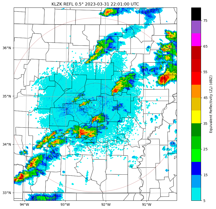
Create a single figure of reflectivity, zoomed into the area of interest.
# Creating color tables for reflectivity (every 5 dBZ starting with 5 dBZ):
ref_norm, ref_cmap = ctables.registry.get_with_steps('NWSReflectivity', 5, 5)
projLCC=ccrs.LambertConformal(central_longitude=cLon, central_latitude=cLat)
sweep = 0
# Call the function that creates the title string, among other things.
timeSweepStr, elevSweepStr = nexRadSweepTimeElev (radar, sweep)
titleStr = f'{site} {shortName} {elevSweepStr} {timeSweepStr}'

# Create our figure
fig = plt.figure(figsize=(15, 10))

# Set up a single axes and plot reflectivity
ax = fig.add_subplot(111, projection=projLCC)
ax.set_extent ([lonW, lonE, latS, latN])

display = pyart.graph.RadarMapDisplay(radar)
ref_map = display.plot_ppi_map(field,sweep=sweep, ax=ax, raster=False, title=titleStr,
            colorbar_label='Equivalent Reflectivity ($Z_{e}$) (dBZ)', norm=ref_norm, cmap=ref_cmap, resolution=res,projection=projLCC,min_lat=latS,max_lat=latN,
                              min_lon=lonW, max_lon=lonE)
range_rings = display.plot_range_rings([10,50,100,200],ax=ax, col='brown',ls='dashed',lw=0.5)

# Add counties
ax.add_feature(USCOUNTIES, linewidth=0.5);
Create a VAD wind profile
# Loop on all sweeps and compute VAD
zlevels = np.arange(100, 5000, 100)  # height above radar
u_allsweeps = []
v_allsweeps = []

#Select only those sweeps that have velocity data
for idx in [1,3,5,6,7,8,10,11,12,13,14,15,16,17,18]:
    print (idx)
    radar_1sweep = radar.extract_sweeps([idx])
    vad = pyart.retrieve.vad_browning(
        radar_1sweep, "velocity", z_want=zlevels
    )
    u_allsweeps.append(vad.u_wind)
    v_allsweeps.append(vad.v_wind)
1
max height 7690.0  meters
min height 17.0  meters
3
max height 9887.0  meters
min height 33.0  meters
5
max height 11498.0  meters
min height 50.0  meters
6
max height 10500.0  meters
min height 67.0  meters
7
max height 11672.0  meters
min height 84.0  meters
8
max height 11071.0  meters
min height 110.0  meters
10
max height 8164.0  meters
min height 20.0  meters
11
max height 11376.0  meters
min height 141.0  meters
12
max height 10816.0  meters
min height 185.0  meters
13
max height 11552.0  meters
min height 234.0  meters
14
max height 11824.0  meters
min height 290.0  meters
15
max height 13388.0  meters
min height 364.0  meters
16
max height 12815.0  meters
min height 456.0  meters
17
max height 12500.0  meters
min height 564.0  meters
18
max height 12595.0  meters
min height 703.0  meters
# Average U and V over all sweeps and compute magnitude and angle
u_avg = np.nanmean(np.array(u_allsweeps), axis=0)
v_avg = np.nanmean(np.array(v_allsweeps), axis=0)
orientation = np.rad2deg(np.arctan2(-u_avg, -v_avg)) % 360
speed = np.sqrt(u_avg**2 + v_avg**2)
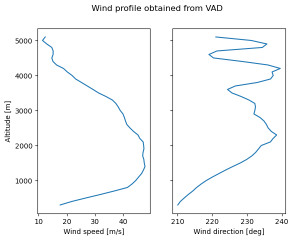
# Display vertical profile of wind
fig, ax = plt.subplots(1, 2, sharey=True)
ax[0].plot(speed * 2, zlevels + radar.altitude["data"])
ax[1].plot(orientation, zlevels + radar.altitude["data"])
ax[0].set_xlabel("Wind speed [m/s]")
ax[1].set_xlabel("Wind direction [deg]")
ax[0].set_ylabel("Altitude [m]")
fig.suptitle("Wind profile obtained from VAD")
Text(0.5, 0.98, 'Wind profile obtained from VAD')