Surface map of METAR data¶

Table of Contents ¶

Objective
Strategy
Step 0: Import required packages
Step 1: Browse a THREDDS Data Server (TDS)
Step 2: Determine the date and hour to gather observations
Step 3: Surface observations

Objective¶

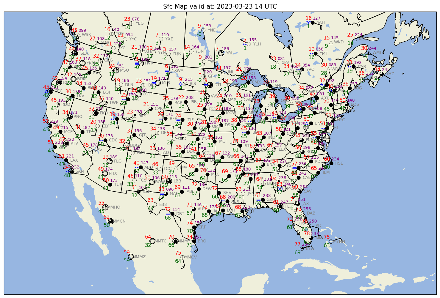
In this notebook, we will make a surface map based on current observations from METAR sites across North America.

Step 0: Import required packages ¶

But first, we need to import all our required packages. Today we’re working with:

datetime

numpy

pandas

matplotlib

cartopy

metpy

siphon

We will also import a couple of functions that convert weather and cloud cover symbols from METAR files encoded in GEMPAK format.

from datetime import datetime,timedelta
import numpy as np
import pandas as pd
import matplotlib.pyplot as plt

import cartopy.crs as ccrs
import cartopy.feature as cfeature

from metpy.calc import wind_components, reduce_point_density
from metpy.units import units
from metpy.plots import StationPlot
from metpy.plots.wx_symbols import current_weather, sky_cover, wx_code_map

from siphon.catalog import TDSCatalog
from siphon.ncss import NCSS

ERROR 1: PROJ: proj_create_from_database: Open of /knight/anaconda_aug22/envs/aug22_env/share/proj failed

# Load in a collection of functions that process GEMPAK weather conditions and cloud cover data.
%run /kt11/ktyle/python/metargem.py

Step 1: Browse a THREDDS Data Server (TDS) ¶

Top

A THREDDS Data Server provides us with coherent access to a large collection of real-time and archived datasets from a variety of environmental data sources at a number of distributed server sites. Various institutions serve data via THREDDS, including our department. You can browse our department’s TDS in your web browser using this link:

http://thredds.atmos.albany.edu:8080/thredds

Let’s take a few moments to browse the catalog in a new tab of your web browser.

Step 2: Determine the date and hour to gather observations ¶

# Use the current time, or set your own for a past time.
# Set current to False if you want to specify a past time.

nowTime = datetime.utcnow()
current = True
#current = False
if (current):
    validTime = datetime.utcnow()
    year = validTime.year
    month = validTime.month
    day = validTime.day
    hour = validTime.hour
else:
    year = 2012
    month = 10
    day = 30
    hour = 0
    
validTime = datetime(year, month, day, hour)
deltaTime = nowTime - validTime
deltaDays = deltaTime.days
timeStr = validTime.strftime("%Y-%m-%d %H UTC")
timeStr2 = validTime.strftime("%Y%m%d%H")

print(timeStr)
print(validTime)
print(deltaTime)
print(deltaDays)

2023-03-23 14 UTC
2023-03-23 14:00:00
0:54:13.556972
0

Step 3: Surface observations ¶

Step 3a: Determine catalog location for Surface observations ¶

Top

If the date is within the past week, use the current METAR data catalog. Otherwise, use the archive METAR data catalog.

if (deltaDays <= 7):
    metar_cat_url = 'http://thredds.atmos.albany.edu:8080/thredds/catalog/metar/ncdecodedNAm/catalog.xml?dataset=metar/ncdecodedNAm/Metar_NAm_Station_Data_fc.cdmr'
else:
    metar_cat_url = 'http://thredds.atmos.albany.edu:8080/thredds/catalog/metarArchive/ncdecoded/catalog.xml?dataset=metarArchive/ncdecoded/Archived_Metar_Station_Data_fc.cdmr'

Note:

Our METAR archive goes back to April 2019. Requests for older dates may fail. If you need data for an earlier date, email Ross or Kevin.

# Create a TDS catalog object from the URL we created above, and examine it.
# The .cdmr extension represents a dataset that works especially well with irregularly-spaced point data sources, such as METAR sites.

catalog = TDSCatalog(metar_cat_url)
catalog

Feature Collection

# This tells us that there is only one dataset type within this catalog, namely a Feature Collection. We now create an object to store this dataset.
metar_dataset = catalog.datasets['Feature Collection']

This dataset consists of multiple hours and locations. We are only interested in a subset of this dataset; for example, the most recent hour, and sites within a geographic domain that we will define below. For this, we will exploit a feature of THREDDS that allows for easy subsetting … the NetCDF Subset Service (NCSS).¶

ncss_url = metar_dataset.access_urls['NetcdfSubset']
print(ncss_url)
# Import ncss client
ncss = NCSS(ncss_url)

http://thredds.atmos.albany.edu:8080/thredds/ncss/metar/ncdecodedNAm/Metar_NAm_Station_Data_fc.cdmr

One of the ncss object’s attributes is variables. Let’s look at that:

ncss.variables

{'ALTI',
 'CEIL',
 'CHC1',
 'CHC2',
 'CHC3',
 'COUN',
 'CTYH',
 'CTYL',
 'CTYM',
 'DRCT',
 'DWPC',
 'GUST',
 'MSUN',
 'P01I',
 'P03C',
 'P03D',
 'P03I',
 'P06I',
 'P24I',
 'PMSL',
 'SKNT',
 'SNEW',
 'SNOW',
 'SPRI',
 'STAT',
 'STD2',
 'STNM',
 'T6NC',
 'T6XC',
 'TDNC',
 'TDXC',
 'TMPC',
 'VSBY',
 'WEQS',
 'WNUM',
 '_isMissing'}

These are abbreviations that the GEMPAK data analysis/visualization package uses for all the meteorological data potentially encoded into a METAR observation.

Step 3b: Subset Surface Observations ¶

Top

Now, let’s request all stations within a bounding box for a given time, select certain variables, and create a surface station plot¶

Make new NCSS query that specifies a regional domain and a particular time.
Request data closest to “now”, or specify a specific YYMMDDHH yourself.
Specify what variables to retreive

# Set the domain to gather data from and for defining the plot region.
latN = 55
latS = 20
lonW = -125
lonE = -60
cLat = (latN + latS)/2
cLon = (lonW + lonE )/2

Step 3c: Retrieve Surface Observations ¶

Top

Create an object to build our data query

query = ncss.query()

query.lonlat_box(north=latN-.25, south=latS+0.5, east=lonE-.25, west=lonW+.25)

# We actually specify a time one minute earlier than the specified hour; this is a quirk of how the data is stored on the THREDDS server and ensures we will get data
# corresponding to the hour we specified
query.time(validTime - timedelta(minutes = 1))

# Select the variables to query.  Note that the variable names depend on the source of the METAR data.
# The 'GEMPAK-like' 4-character names are from the UAlbany THREDDS.

query.variables('TMPC', 'DWPC', 'PMSL',
                'SKNT', 'DRCT','ALTI','WNUM','VSBY','CHC1', 'CHC2', 'CHC3','CTYH', 'CTYM', 'CTYL' )
query.accept('csv')

var=WNUM&var=CHC2&var=CTYH&var=PMSL&var=ALTI&var=DRCT&var=TMPC&var=DWPC&var=VSBY&var=CTYL&var=CHC1&var=CTYM&var=CHC3&var=SKNT&time=2023-03-23T13%3A59%3A00&west=-124.75&east=-60.25&south=20.5&north=54.75&accept=csv

Pass the query to the THREDDS server’s NCSS service. We can then create a Pandas dataframe from the returned object.

data = ncss.get_data(query)
df = pd.DataFrame(data)
df

/knight/anaconda_aug22/envs/aug22_env/lib/python3.10/site-packages/siphon/ncss.py:432: VisibleDeprecationWarning: Reading unicode strings without specifying the encoding argument is deprecated. Set the encoding, use None for the system default.
  arrs = np.genfromtxt(fobj, dtype=None, names=names, delimiter=',',

	time	station	latitude	longitude	WNUM	CHC2	CTYH	PMSL	ALTI	DRCT	TMPC	DWPC	VSBY	CTYL	CHC1	CTYM	CHC3	SKNT
0	b'2023-03-23T14:00:00Z'	b'ABI'	32.419	-99.680	NaN	NaN	NaN	1011.10004	29.929998	NaN	20.6	17.2	10.0	NaN	194.0	NaN	NaN	3.0
1	b'2023-03-23T14:00:00Z'	b'ABQ'	35.049	-106.620	13.0	NaN	NaN	1014.70000	30.039999	120.0	4.4	0.0	10.0	NaN	324.0	NaN	NaN	7.0
2	b'2023-03-23T14:00:00Z'	b'AEX'	31.329	-92.550	9.0	154.0	NaN	1020.00000	30.109999	150.0	20.0	18.9	5.0	NaN	73.0	NaN	NaN	7.0
3	b'2023-03-23T14:00:00Z'	b'ALB'	42.750	-73.800	NaN	NaN	NaN	1011.90000	29.880000	160.0	10.0	7.2	10.0	NaN	554.0	NaN	NaN	6.0
4	b'2023-03-23T14:00:00Z'	b'ANJ'	46.479	-84.370	NaN	NaN	NaN	1011.90000	29.859999	310.0	-1.1	-6.1	10.0	NaN	244.0	NaN	NaN	16.0
...	...	...	...	...	...	...	...	...	...	...	...	...	...	...	...	...	...	...
179	b'2023-03-23T14:00:00Z'	b'YXE'	52.169	-106.680	NaN	NaN	NaN	1011.00000	29.730000	180.0	-14.0	-16.0	15.0	NaN	1.0	NaN	NaN	8.0
180	b'2023-03-23T14:00:00Z'	b'YXH'	50.020	-110.720	NaN	NaN	NaN	1011.00000	29.750000	200.0	-6.0	-11.0	30.0	NaN	1.0	NaN	NaN	10.0
181	b'2023-03-23T14:00:00Z'	b'YYC'	51.119	-114.019	NaN	NaN	1.0	1009.40000	29.660000	210.0	-6.0	-12.0	30.0	0.0	2206.0	0.0	NaN	5.0
182	b'2023-03-23T14:00:00Z'	b'YYN'	50.279	-107.680	NaN	NaN	NaN	1012.10004	29.740000	210.0	-7.0	-12.0	9.0	NaN	1.0	NaN	NaN	19.0
183	b'2023-03-23T14:00:00Z'	b'YYZ'	43.669	-79.599	733.0	154.0	0.0	1008.90000	29.779999	300.0	7.0	7.0	2.0	7.0	52.0	0.0	NaN	7.0

184 rows × 18 columns

Step 3d: Process Surface Observations ¶

Top

Read in several of the columns; assign / convert units as necessary; convert GEMPAK cloud cover and present wx symbols to MetPy’s representation¶

lats = data['latitude']
lons = data['longitude']
tair = (data['TMPC'] * units ('degC')).to('degF')
dewp = (data['DWPC'] * units ('degC')).to('degF')
altm = (data['ALTI'] * units('inHg')).to('mbar')
slp = data['PMSL']

# Convert wind to components
u, v = wind_components(data['SKNT'] * units.knots, data['DRCT'] * units.degree)

# replace missing wx codes or those >= 100 with 0, and convert to MetPy's present weather code
wnum = (np.nan_to_num(data['WNUM'],True).astype(int))
convert_wnum (wnum)



# Need to handle missing (NaN) and convert to proper code
chc1 = (np.nan_to_num(data['CHC1'],True).astype(int))
chc2 = (np.nan_to_num(data['CHC2'],True).astype(int))
chc3 = (np.nan_to_num(data['CHC3'],True).astype(int))
cloud_cover = calc_clouds(chc1, chc2, chc3)

# For some reason station id's come back as bytes instead of strings. This line converts the array of station id's into an array of strings.
stid = np.array([s.decode() for s in data['station']])

The next step deals with the removal of overlapping stations, using reduce_point_density. This returns a mask we can apply to data to filter the points.

# Project points so that we're filtering based on the way the stations are laid out on the map
proj = ccrs.Stereographic(central_longitude=cLon, central_latitude=cLat)
xy = proj.transform_points(ccrs.PlateCarree(), lons, lats)

# Reduce point density so that there's only one point within a circle whose distance is specified in meters.
# This value will need to change depending on how large of an area you are plotting.
density = 100000
mask = reduce_point_density(xy, density)

Step 3e: Visualize Surface Observations ¶

Top

Simple station plotting using plot methods¶

One way to create station plots with MetPy is to create an instance of StationPlot and call various plot methods, like plot_parameter, to plot arrays of data at locations relative to the center point.

In addition to plotting values, StationPlot has support for plotting text strings, symbols, and plotting values using custom formatting.

Plotting symbols involves mapping integer values to various custom font glyphs in our custom weather symbols font. MetPy provides mappings for converting WMO codes to their appropriate symbol. The sky_cover and current_weather functions below are two such mappings.

Now we just plot with arr[mask] for every arr of data we use in plotting.

# Set up a plot with map features
# First set dpi ("dots per inch") - higher values will give us a less pixelated final figure.
dpi = 125

fig = plt.figure(figsize=(15,10), dpi=dpi)

proj = ccrs.Stereographic(central_longitude=cLon, central_latitude=cLat)
ax = fig.add_subplot(1, 1, 1, projection=proj)
ax.set_facecolor(cfeature.COLORS['water'])

land_mask = cfeature.NaturalEarthFeature('physical', 'land', '50m',
                                        edgecolor='face',
                                        facecolor=cfeature.COLORS['land'])
lake_mask = cfeature.NaturalEarthFeature('physical', 'lakes', '50m',
                                        edgecolor='face',
                                        facecolor=cfeature.COLORS['water'])
state_borders = cfeature.NaturalEarthFeature(category='cultural', name='admin_1_states_provinces_lakes',
                                         scale='50m', facecolor='none')

ax.add_feature(land_mask)
ax.add_feature(lake_mask)
ax.add_feature(state_borders, linestyle='solid', edgecolor='black')

# Slightly reduce the extent of the map as compared to the subsetted data region; this helps eliminate data from being plotted beyond the frame of the map
ax.set_extent ((lonW+2,lonE-4,latS-1,latN-2), crs=ccrs.PlateCarree())


#If we wanted to add grid lines to our plot:
#ax.gridlines()

# Create a station plot pointing to an Axes to draw on as well as the location of points
stationplot = StationPlot(ax, lons[mask], lats[mask], transform=ccrs.PlateCarree(),
                          fontsize=8)

stationplot.plot_parameter('NW', tair[mask], color='red', fontsize=10)
stationplot.plot_parameter('SW', dewp[mask], color='darkgreen', fontsize=10)

# Below, we are using a custom formatter to control how the sea-level pressure
# values are plotted. This uses the standard trailing 3-digits of the pressure value
# in tenths of millibars.
stationplot.plot_parameter('NE', slp[mask], color='purple', formatter=lambda v: format(10 * v, '.0f')[-3:])



stationplot.plot_symbol('C', cloud_cover[mask], sky_cover)
stationplot.plot_symbol('W', wnum[mask], current_weather,color='blue',fontsize=12)
stationplot.plot_text((2, 0),stid[mask], color='gray')
#zorder - Higher value zorder will plot the variable on top of lower value zorder. This is necessary for wind barbs to appear. Default is 1.
stationplot.plot_barb(u[mask], v[mask],zorder=2)

plt.title("Sfc Map valid at: "+ timeStr)
plt.savefig (timeStr2 + '_sfmap.png',dpi=dpi)

../../_images/01_Metpy_MetarPlot_37_0.png

# In order to see the entire figure, type the name of the figure object below.
fig

../../_images/01_Metpy_MetarPlot_38_0.png

ATM350 Spring 2023

Surface map of METAR data

Contents