Skew-T’s
Contents
Skew-T’s
Requesting Upper Air Data from Siphon and Plotting a Skew-T with MetPy
Based on Unidata’s MetPy Monday # 15 -17 YouTube links:
https://www.youtube.com/watch?v=OUTBiXEuDIU;
https://www.youtube.com/watch?v=oog6_b-844Q;
https://www.youtube.com/watch?v=b0RsN9mCY5k
Import the libraries we need
import numpy as np
import matplotlib.pyplot as plt
from mpl_toolkits.axes_grid1.inset_locator import inset_axes
import metpy.calc as mpcalc
from metpy.plots import Hodograph, SkewT
from metpy.units import units, pandas_dataframe_to_unit_arrays
from datetime import datetime, timedelta
import pandas as pd
from siphon.simplewebservice.wyoming import WyomingUpperAir
ERROR 1: PROJ: proj_create_from_database: Open of /knight/anaconda_aug22/envs/aug22_env/share/proj failed
Next we use methods from the datetime library to determine the latest time, and then use it to select the most recent date and time that we’ll use for our selected Skew-T.
now = datetime.utcnow()

curr_year = now.year
curr_month = now.month
curr_day = now.day
curr_hour = now.hour

print("Current time is: ", now)
print("Current year, month, date, hour: " ,curr_year, curr_month,curr_day,curr_hour)

if (curr_hour > 13) :
    raob_hour = 12
    hr_delta = curr_hour - 12
elif (curr_hour > 1):
    raob_hour = 0
    hr_delta = curr_hour - 0
else:
    raob_hour = 12
    hr_delta = curr_hour + 12

raob_time = now - timedelta(hours=hr_delta)

raob_year = raob_time.year
raob_month = raob_time.month
raob_day = raob_time.day
raob_hour = raob_time.hour

print("Time of RAOB is: ", raob_year, raob_month, raob_day, raob_hour)
Current time is:  2023-03-28 18:46:23.406966
Current year, month, date, hour:  2023 3 28 18
Time of RAOB is:  2023 3 28 12
Construct a datetime object that we will use in our query to the data server. Note what it looks like.
query_date = datetime(raob_year,raob_month,raob_day,raob_hour)
query_date
datetime.datetime(2023, 3, 28, 12, 0)
If desired, we can choose a past date and time.
#current = True
current = False
if (current == False):
    query_date = datetime(2012, 10, 29, 12)

raob_timeStr = query_date.strftime("%Y-%m-%d %H UTC")
raob_timeTitle = query_date.strftime("%H00 UTC %-d %b %Y")
print(raob_timeStr)
print(raob_timeTitle)
2012-10-29 12 UTC
1200 UTC 29 Oct 2012
Select our station and query the data server.
station = 'ALB'

df = WyomingUpperAir.request_data (query_date,station)
What does the returned data file look like? Well, it looks like a Pandas Dataframe!
df
| pressure | height | temperature | dewpoint | direction | speed | u_wind | v_wind | station | station_number | time | latitude | longitude | elevation | pw | |
|---|---|---|---|---|---|---|---|---|---|---|---|---|---|---|---|
| 0 | 993.0 | 96 | 12.6 | 7.6 | 0.0 | 8.0 | -0.000000 | -8.000000e+00 | ALB | 72518 | 2012-10-29 12:00:00 | 42.7 | -73.83 | 96.0 | 16.8 |
| 1 | 990.0 | 122 | 12.0 | 7.0 | 2.0 | 10.0 | -0.348995 | -9.993908e+00 | ALB | 72518 | 2012-10-29 12:00:00 | 42.7 | -73.83 | 96.0 | 16.8 |
| 2 | 968.6 | 305 | 10.4 | 6.5 | 20.0 | 25.0 | -8.550504 | -2.349232e+01 | ALB | 72518 | 2012-10-29 12:00:00 | 42.7 | -73.83 | 96.0 | 16.8 |
| 3 | 955.0 | 423 | 9.4 | 6.1 | 26.0 | 26.0 | -11.397650 | -2.336865e+01 | ALB | 72518 | 2012-10-29 12:00:00 | 42.7 | -73.83 | 96.0 | 16.8 |
| 4 | 933.8 | 610 | 8.1 | 5.7 | 35.0 | 27.0 | -15.486564 | -2.211711e+01 | ALB | 72518 | 2012-10-29 12:00:00 | 42.7 | -73.83 | 96.0 | 16.8 |
| ... | ... | ... | ... | ... | ... | ... | ... | ... | ... | ... | ... | ... | ... | ... | ... |
| 138 | 10.4 | 30480 | -57.3 | NaN | 295.0 | 22.0 | 19.938771 | -9.297602e+00 | ALB | 72518 | 2012-10-29 12:00:00 | 42.7 | -73.83 | 96.0 | 16.8 |
| 139 | 10.0 | 30720 | -58.1 | NaN | 280.0 | 23.0 | 22.650578 | -3.993908e+00 | ALB | 72518 | 2012-10-29 12:00:00 | 42.7 | -73.83 | 96.0 | 16.8 |
| 140 | 9.7 | 30911 | -58.9 | NaN | 277.0 | 26.0 | 25.806200 | -3.168603e+00 | ALB | 72518 | 2012-10-29 12:00:00 | 42.7 | -73.83 | 96.0 | 16.8 |
| 141 | 9.0 | 31394 | -58.2 | NaN | 270.0 | 34.0 | 34.000000 | 6.245699e-15 | ALB | 72518 | 2012-10-29 12:00:00 | 42.7 | -73.83 | 96.0 | 16.8 |
| 142 | 8.7 | 31595 | -57.9 | NaN | NaN | NaN | NaN | NaN | ALB | 72518 | 2012-10-29 12:00:00 | 42.7 | -73.83 | 96.0 | 16.8 |
143 rows × 15 columns
We need to deal with an issue where two levels may be at the same pressure, but different heights. While rare, it won’t allow a parcel path to be calculated later in this notebook:
We can check to see if this is occurring by looking more closely at the data. Let’s look at the last 30 rows of this dataframe (this issue usually occurs near the very top, or lowest pressures, of our sounding data:
df.tail(30)
| pressure | height | temperature | dewpoint | direction | speed | u_wind | v_wind | station | station_number | time | latitude | longitude | elevation | pw | |
|---|---|---|---|---|---|---|---|---|---|---|---|---|---|---|---|
| 113 | 42.4 | 21641 | -63.3 | -88.2 | 150.0 | 1.0 | -0.500000 | 8.660254e-01 | ALB | 72518 | 2012-10-29 12:00:00 | 42.7 | -73.83 | 96.0 | 16.8 |
| 114 | 42.3 | 21654 | -63.3 | -88.3 | 149.0 | 1.0 | -0.515038 | 8.571673e-01 | ALB | 72518 | 2012-10-29 12:00:00 | 42.7 | -73.83 | 96.0 | 16.8 |
| 115 | 40.5 | 21923 | -60.9 | -90.9 | 131.0 | 6.0 | -4.528257 | 3.936354e+00 | ALB | 72518 | 2012-10-29 12:00:00 | 42.7 | -73.83 | 96.0 | 16.8 |
| 116 | 38.0 | 22319 | -61.1 | NaN | 105.0 | 13.0 | -12.557036 | 3.364648e+00 | ALB | 72518 | 2012-10-29 12:00:00 | 42.7 | -73.83 | 96.0 | 16.8 |
| 117 | 36.8 | 22520 | -58.3 | NaN | 92.0 | 16.0 | -15.990253 | 5.583919e-01 | ALB | 72518 | 2012-10-29 12:00:00 | 42.7 | -73.83 | 96.0 | 16.8 |
| 118 | 36.6 | 22555 | -58.3 | NaN | 90.0 | 17.0 | -17.000000 | -1.040950e-15 | ALB | 72518 | 2012-10-29 12:00:00 | 42.7 | -73.83 | 96.0 | 16.8 |
| 119 | 34.9 | 22860 | -57.9 | NaN | 125.0 | 12.0 | -9.829825 | 6.882917e+00 | ALB | 72518 | 2012-10-29 12:00:00 | 42.7 | -73.83 | 96.0 | 16.8 |
| 120 | 33.2 | 23165 | -57.5 | NaN | 105.0 | 10.0 | -9.659258 | 2.588190e+00 | ALB | 72518 | 2012-10-29 12:00:00 | 42.7 | -73.83 | 96.0 | 16.8 |
| 121 | 31.7 | 23470 | -57.1 | NaN | 135.0 | 11.0 | -7.778175 | 7.778175e+00 | ALB | 72518 | 2012-10-29 12:00:00 | 42.7 | -73.83 | 96.0 | 16.8 |
| 122 | 31.7 | 23462 | -57.1 | NaN | 134.0 | 11.0 | -7.912738 | 7.641242e+00 | ALB | 72518 | 2012-10-29 12:00:00 | 42.7 | -73.83 | 96.0 | 16.8 |
| 123 | 30.0 | 23810 | -57.9 | NaN | 45.0 | 9.0 | -6.363961 | -6.363961e+00 | ALB | 72518 | 2012-10-29 12:00:00 | 42.7 | -73.83 | 96.0 | 16.8 |
| 124 | 27.4 | 24384 | -58.3 | NaN | 85.0 | 9.0 | -8.965752 | -7.844017e-01 | ALB | 72518 | 2012-10-29 12:00:00 | 42.7 | -73.83 | 96.0 | 16.8 |
| 125 | 26.2 | 24663 | -58.5 | NaN | 66.0 | 10.0 | -9.135455 | -4.067366e+00 | ALB | 72518 | 2012-10-29 12:00:00 | 42.7 | -73.83 | 96.0 | 16.8 |
| 126 | 24.0 | 25212 | -61.1 | NaN | 29.0 | 11.0 | -5.332906 | -9.620817e+00 | ALB | 72518 | 2012-10-29 12:00:00 | 42.7 | -73.83 | 96.0 | 16.8 |
| 127 | 20.8 | 26104 | -59.9 | NaN | 327.0 | 14.0 | 7.624946 | -1.174139e+01 | ALB | 72518 | 2012-10-29 12:00:00 | 42.7 | -73.83 | 96.0 | 16.8 |
| 128 | 20.4 | 26213 | -59.1 | NaN | 320.0 | 14.0 | 8.999027 | -1.072462e+01 | ALB | 72518 | 2012-10-29 12:00:00 | 42.7 | -73.83 | 96.0 | 16.8 |
| 129 | 20.0 | 26350 | -58.1 | NaN | 335.0 | 14.0 | 5.916656 | -1.268831e+01 | ALB | 72518 | 2012-10-29 12:00:00 | 42.7 | -73.83 | 96.0 | 16.8 |
| 130 | 19.5 | 26518 | -58.2 | NaN | 345.0 | 14.0 | 3.623467 | -1.352296e+01 | ALB | 72518 | 2012-10-29 12:00:00 | 42.7 | -73.83 | 96.0 | 16.8 |
| 131 | 18.6 | 26822 | -58.3 | NaN | 350.0 | 10.0 | 1.736482 | -9.848078e+00 | ALB | 72518 | 2012-10-29 12:00:00 | 42.7 | -73.83 | 96.0 | 16.8 |
| 132 | 17.7 | 27127 | -58.4 | NaN | 280.0 | 5.0 | 4.924039 | -8.682409e-01 | ALB | 72518 | 2012-10-29 12:00:00 | 42.7 | -73.83 | 96.0 | 16.8 |
| 133 | 16.8 | 27432 | -58.5 | NaN | 290.0 | 9.0 | 8.457234 | -3.078181e+00 | ALB | 72518 | 2012-10-29 12:00:00 | 42.7 | -73.83 | 96.0 | 16.8 |
| 134 | 16.7 | 27483 | -58.5 | NaN | 290.0 | 9.0 | 8.457234 | -3.078181e+00 | ALB | 72518 | 2012-10-29 12:00:00 | 42.7 | -73.83 | 96.0 | 16.8 |
| 135 | 14.6 | 28332 | -56.1 | NaN | 291.0 | 13.0 | 12.136546 | -4.658783e+00 | ALB | 72518 | 2012-10-29 12:00:00 | 42.7 | -73.83 | 96.0 | 16.8 |
| 136 | 12.4 | 29363 | -58.3 | NaN | 293.0 | 17.0 | 15.648583 | -6.642429e+00 | ALB | 72518 | 2012-10-29 12:00:00 | 42.7 | -73.83 | 96.0 | 16.8 |
| 137 | 10.7 | 30293 | -56.7 | NaN | 295.0 | 21.0 | 19.032464 | -8.874983e+00 | ALB | 72518 | 2012-10-29 12:00:00 | 42.7 | -73.83 | 96.0 | 16.8 |
| 138 | 10.4 | 30480 | -57.3 | NaN | 295.0 | 22.0 | 19.938771 | -9.297602e+00 | ALB | 72518 | 2012-10-29 12:00:00 | 42.7 | -73.83 | 96.0 | 16.8 |
| 139 | 10.0 | 30720 | -58.1 | NaN | 280.0 | 23.0 | 22.650578 | -3.993908e+00 | ALB | 72518 | 2012-10-29 12:00:00 | 42.7 | -73.83 | 96.0 | 16.8 |
| 140 | 9.7 | 30911 | -58.9 | NaN | 277.0 | 26.0 | 25.806200 | -3.168603e+00 | ALB | 72518 | 2012-10-29 12:00:00 | 42.7 | -73.83 | 96.0 | 16.8 |
| 141 | 9.0 | 31394 | -58.2 | NaN | 270.0 | 34.0 | 34.000000 | 6.245699e-15 | ALB | 72518 | 2012-10-29 12:00:00 | 42.7 | -73.83 | 96.0 | 16.8 |
| 142 | 8.7 | 31595 | -57.9 | NaN | NaN | NaN | NaN | NaN | ALB | 72518 | 2012-10-29 12:00:00 | 42.7 | -73.83 | 96.0 | 16.8 |
If any rows have the same pressure, this will cause an error when we call MetPy’s parcel_path function. Likely this will get resolved in a future release of MetPy, but for now, let’s use a Pandas function to eliminate rows whose pressure is the same as a previous row.
df.drop_duplicates(inplace=True,subset='pressure',ignore_index=True)
df['pressure']
0      993.0
1      990.0
2      968.6
3      955.0
4      933.8
       ...
137     10.4
138     10.0
139      9.7
140      9.0
141      8.7
Name: pressure, Length: 142, dtype: float64
As with any Pandas Dataframe, we can select columns, so we do so now for all the relevant variables for our Skew-T. Note now that we are using MetPy’s units library to attach units to each variable’s array of values.
p = df['pressure'].values * units(df.units['pressure'])
#Let's split up the code above, to see more detail:
df['pressure'].values
array([993. , 990. , 968.6, 955. , 933.8, 925. , 900. , 876. , 867.1,
       850. , 833. , 818. , 813. , 806. , 804.2, 794. , 783. , 774.5,
       754. , 746. , 740. , 718.4, 716. , 706. , 700. , 690. , 680. ,
       666. , 663. , 649. , 641.1, 640. , 630. , 596. , 593.9, 584. ,
       550. , 549.5, 517. , 508. , 500. , 493. , 490. , 486. , 484. ,
       477. , 472. , 469.3, 466. , 458. , 451. , 446. , 437. , 432.9,
       428. , 427. , 419. , 409. , 404. , 400. , 398. , 388. , 383.1,
       380. , 331. , 318. , 310.6, 300. , 250. , 217. , 216.8, 205. ,
       200. , 198. , 183. , 172. , 166. , 162.6, 160. , 154.8, 153. ,
       151. , 150. , 145. , 143. , 140.2, 134. , 120.8, 118. , 105. ,
       100. ,  96. ,  87.1,  81.6,  80.9,  76.2,  73.3,  73.2,  72.5,
        70. ,  68.6,  66.2,  63. ,  60. ,  58.7,  54.2,  51.6,  50.2,
        50. ,  49. ,  47.1,  46.8,  44.5,  42.4,  42.3,  40.5,  38. ,
        36.8,  36.6,  34.9,  33.2,  31.7,  30. ,  27.4,  26.2,  24. ,
        20.8,  20.4,  20. ,  19.5,  18.6,  17.7,  16.8,  16.7,  14.6,
        12.4,  10.7,  10.4,  10. ,   9.7,   9. ,   8.7])
The University of Wyoming sounding reader includes a units attribute, which produces a Python dictionary of units specific to Wyoming sounding data. What does it look like?
df.units
{'pressure': 'hPa',
 'height': 'meter',
 'temperature': 'degC',
 'dewpoint': 'degC',
 'direction': 'degrees',
 'speed': 'knot',
 'u_wind': 'knot',
 'v_wind': 'knot',
 'station': None,
 'station_number': None,
 'time': None,
 'latitude': 'degrees',
 'longitude': 'degrees',
 'elevation': 'meter',
 'pw': 'millimeter'}
#From the dictionary, we can specify pressure units.  In this case, hectopascal (hPa):
units(df.units['pressure'])
#Putting it all together...
p
| Magnitude | [993.0 990.0 968.6 955.0 933.8 925.0 900.0 876.0 867.1 850.0 833.0 818.0 |
|---|---|
| Units | hectopascal |
#set this for use later:
p_units=units(df.units['pressure'])
#Set remaining variables and apply units:
Z = df['height'].values * units(df.units['height'])
T = df['temperature'].values * units(df.units['temperature'])
Td = df['dewpoint'].values * units(df.units['dewpoint'])
u = df['u_wind'].values * units(df.units['u_wind'])
v = df['v_wind'].values * units(df.units['v_wind'])
Note: we can also attach units to the various columns using MetPy’s pandas_dataframe_to_unit_arrays function, as follows:
df = pandas_dataframe_to_unit_arrays(df)
Now that u and v are units aware, we can use one of MetPy’s diagnostic routines to calculate the wind speed from the vector’s components.
wind_speed = mpcalc.wind_speed(u,v)
Thermodynamic Calculations
Often times we will want to calculate some thermodynamic parameters of a sounding. The MetPy calc module has many such calculations already implemented!
Lifting Condensation Level (LCL) - The level at which an air parcel’s relative humidity becomes 100% when lifted along a dry adiabatic path.
Parcel Path - Path followed by a hypothetical parcel of air, beginning at the surface temperature/pressure and rising dry adiabatically until reaching the LCL, then rising moist adiabatially.
Calculate the LCL. Note that the units will appear at the end when we print them out!
lclp, lclt = mpcalc.lcl(p[0], T[0], Td[0])
print ('LCL Pressure = ',lclp, 'LCL Temperature = ',lclt)
LCL Pressure = 920.7394732770757 hectopascal LCL Temperature = 6.497694364794597 degree_Celsius
Calculate the parcel profile. Here, we pass in the array of all pressure values, and specify the first (index 0, remember Python’s zero-based indexing) index of the temperature and dewpoint arrays as the starting point of the parcel path.
parcel_prof = mpcalc.parcel_profile(p, T[0], Td[0])
What does the parcel profile look like? Well, it’s just an array of all the temperatures of the parcel at each of the pressure levels as it ascends.
parcel_prof
| Magnitude | [285.75 285.50307824573736 283.7260147751601 282.5820425453529 |
|---|---|
| Units | kelvin |
Set the limits for the x- and y-axes so they can be changed and easily re-used when desired.
pTop = 100
pBot = 1050
tMin = -60
tMax = 40
Since we are plotting a skew-T, define the log-p axis.
logTop = np.log10(pTop)
logBot = np.log10(pBot)
interval = np.logspace(logTop,logBot) * p_units
This interval will tend to oversample points near the top of the atmosphere relative to the bottom. One effect of this will be that wind barbs will be hard to read, especially at higher levels. Use a resampling method from NumPy to deal with this.
idx = mpcalc.resample_nn_1d(p, interval)
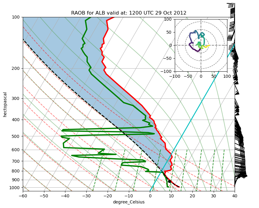
Now we are ready to create our skew-T. Plot it and save it as a PNG file.
Note:
Annoyingly, when specifying the color of the dry/moist adiabats, and mixing ratio lines, the parameter must be colors, not color. In other Matplotlib-related code lines in the cell below where we set the color, such as skew.ax.axvline , color must be singular.
# Create a new figure. The dimensions here give a good aspect ratio
fig = plt.figure(figsize=(9, 9))
skew = SkewT(fig, rotation=30)

# Plot the data using normal plotting functions, in this case using
# log scaling in Y, as dictated by the typical meteorological plot
skew.plot(p, T, 'r', linewidth=3)
skew.plot(p, Td, 'g', linewidth=3)
skew.plot_barbs(p[idx], u[idx], v[idx])
skew.ax.set_ylim(pBot, pTop)
skew.ax.set_xlim(tMin, tMax)

# Plot LCL as black dot
skew.plot(lclp, lclt, 'ko', markerfacecolor='black')

# Plot the parcel profile as a black line
skew.plot(p, parcel_prof, 'k', linestyle='--', linewidth=2)

# Shade areas of CAPE and CIN
skew.shade_cin(p, T, parcel_prof)
skew.shade_cape(p, T, parcel_prof)

# Plot a zero degree isotherm
skew.ax.axvline(0, color='c', linestyle='-', linewidth=2)

# Add the relevant special lines
skew.plot_dry_adiabats()
skew.plot_moist_adiabats(colors='#58a358', linestyle='-')
skew.plot_mixing_lines()

plt.title("RAOB for " + station + ' valid at: '+ raob_timeTitle)

# Create a hodograph
# Create an inset axes object that is 30% width and height of the
# figure and put it in the upper right hand corner.
ax_hod = inset_axes(skew.ax, '30%', '30%', loc=1)
h = Hodograph(ax_hod, component_range=100.)
h.add_grid(increment=30)
#h.plot_colormapped(u, v, df['height'].values)  # Plot a line colored by a parameter
h.plot_colormapped(u, v, df['height'])
plt.savefig (station + raob_timeStr + '_skewt.png')
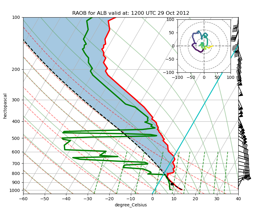
Here’s how the plot would appear if we hadn’t done the resampling. Note that the wind barbs are plotted at every level, and are harder to read:
# Create a new figure. The dimensions here give a good aspect ratio
fig = plt.figure(figsize=(9, 9))
skew = SkewT(fig, rotation=30)

# Plot the data using normal plotting functions, in this case using
# log scaling in Y, as dictated by the typical meteorological plot
skew.plot(p, T, 'r', linewidth=3)
skew.plot(p, Td, 'g', linewidth=3)
skew.plot_barbs(p, u, v)
skew.ax.set_ylim(pBot, pTop)
skew.ax.set_xlim(tMin, tMax)

# Plot LCL as black dot
skew.plot(lclp, lclt, 'ko', markerfacecolor='black')

# Plot the parcel profile as a black line
skew.plot(p, parcel_prof, 'k', linestyle='--', linewidth=2)

# Shade areas of CAPE and CIN
skew.shade_cin(p, T, parcel_prof)
skew.shade_cape(p, T, parcel_prof)

# Plot a zero degree isotherm
skew.ax.axvline(0, color='c', linestyle='-', linewidth=2)

# Add the relevant special lines
skew.plot_dry_adiabats()
skew.plot_moist_adiabats(colors='#58a358', linestyle='-')
skew.plot_mixing_lines()

plt.title("RAOB for " + station + ' valid at: '+ raob_timeTitle)

# Create a hodograph
# Create an inset axes object that is 30% width and height of the
# figure and put it in the upper right hand corner.
ax_hod = inset_axes(skew.ax, '30%', '30%', loc=1)
h = Hodograph(ax_hod, component_range=100.)
h.add_grid(increment=30)
h.plot_colormapped(u, v, df['height'])  # Plot a line colored by a parameter
<matplotlib.collections.LineCollection at 0x151dca71dab0>