NYSM_TimeSeries.ipynb
Contents
NYSM_TimeSeries.ipynb
This notebook generates time series of recent meteorological data for various New York State Mesonet (NYSM) sites.
TRY THIS: Edit the next Markdown cell with your first and last name.
Author: firstName lastName
Imports
from datetime import datetime
import pandas as pd
import matplotlib.pyplot as plt
import seaborn as sns
Create a Pandas DataFrame to read in the file containing the past hour’s worth of NYSM data.
# First define the format and then define the lambda function
timeFormat = "%Y-%m-%d %H:%M:%S UTC"
# This function will iterate over each string in a 1-d array
# and use Pandas' implementation of strptime to convert the string into a datetime object.
parseTime = lambda x: datetime.strptime(x, timeFormat)
df = pd.read_csv('/data1/nysm/latest.csv',parse_dates=['time'], date_parser=parseTime).set_index('time')
Inspect the Dataframe.
df
| station | temp_2m [degC] | temp_9m [degC] | relative_humidity [percent] | precip_incremental [mm] | precip_local [mm] | precip_max_intensity [mm/min] | avg_wind_speed_prop [m/s] | max_wind_speed_prop [m/s] | wind_speed_stddev_prop [m/s] | ... | snow_depth [cm] | frozen_soil_05cm [bit] | frozen_soil_25cm [bit] | frozen_soil_50cm [bit] | soil_temp_05cm [degC] | soil_temp_25cm [degC] | soil_temp_50cm [degC] | soil_moisture_05cm [m^3/m^3] | soil_moisture_25cm [m^3/m^3] | soil_moisture_50cm [m^3/m^3] | |
|---|---|---|---|---|---|---|---|---|---|---|---|---|---|---|---|---|---|---|---|---|---|
| time | |||||||||||||||||||||
| 2023-02-15 02:40:00 | ADDI | 5.2 | 5.9 | 43.4 | 0.0 | 0.0 | 0.0 | 5.3 | 6.7 | 0.7 | ... | -1.0 | 0.0 | 0.0 | 0.0 | 0.8 | 1.6 | 2.2 | 0.54 | 0.44 | 0.43 |
| 2023-02-15 02:45:00 | ADDI | 5.2 | 5.9 | 43.3 | 0.0 | 0.0 | 0.0 | 4.4 | 6.6 | 0.7 | ... | -1.0 | 0.0 | 0.0 | 0.0 | 0.8 | 1.6 | 2.2 | 0.54 | 0.44 | 0.43 |
| 2023-02-15 02:50:00 | ADDI | 5.1 | 5.8 | 43.8 | 0.0 | 0.0 | 0.0 | 4.6 | 5.7 | 0.5 | ... | -1.0 | 0.0 | 0.0 | 0.0 | 0.8 | 1.6 | 2.2 | 0.54 | 0.44 | 0.43 |
| 2023-02-15 02:55:00 | ADDI | 4.9 | 5.6 | 44.3 | 0.0 | 0.0 | 0.0 | 4.1 | 5.4 | 0.5 | ... | -1.0 | 0.0 | 0.0 | 0.0 | 0.8 | 1.6 | 2.2 | 0.54 | 0.44 | 0.43 |
| 2023-02-15 03:00:00 | ADDI | 4.9 | 5.5 | 45.0 | 0.0 | 0.0 | 0.0 | 4.1 | 5.6 | 0.6 | ... | -1.0 | 0.0 | 0.0 | 0.0 | 0.8 | 1.6 | 2.2 | 0.54 | 0.44 | 0.43 |
| ... | ... | ... | ... | ... | ... | ... | ... | ... | ... | ... | ... | ... | ... | ... | ... | ... | ... | ... | ... | ... | ... |
| 2023-02-15 03:20:00 | YORK | 0.9 | 2.4 | 80.1 | 0.0 | 0.0 | 0.0 | 0.1 | 0.5 | 0.1 | ... | 0.0 | 0.0 | 0.0 | 0.0 | 3.0 | 3.1 | 3.0 | 0.26 | 0.29 | 0.34 |
| 2023-02-15 03:25:00 | YORK | 1.2 | 2.1 | 77.5 | 0.0 | 0.0 | 0.0 | 0.0 | 0.4 | 0.1 | ... | 0.0 | 0.0 | 0.0 | 0.0 | 3.0 | 3.1 | 3.0 | 0.26 | 0.29 | 0.34 |
| 2023-02-15 03:30:00 | YORK | 0.7 | 1.9 | 82.4 | 0.0 | 0.0 | 0.0 | 0.0 | 0.0 | 0.0 | ... | 0.0 | 0.0 | 0.0 | 0.0 | 3.0 | 3.1 | 3.0 | 0.26 | 0.29 | 0.34 |
| 2023-02-15 03:35:00 | YORK | 0.5 | 1.8 | 82.0 | 0.0 | 0.0 | 0.0 | 0.0 | 0.0 | 0.0 | ... | 0.0 | 0.0 | 0.0 | 0.0 | 3.0 | 3.1 | 3.0 | 0.26 | 0.29 | 0.34 |
| 2023-02-15 03:40:00 | YORK | 0.7 | 2.1 | 81.4 | 0.0 | 0.0 | 0.0 | 0.3 | 0.9 | 0.3 | ... | 0.0 | 0.0 | 0.0 | 0.0 | 3.0 | 3.1 | 3.0 | 0.26 | 0.29 | 0.34 |
1638 rows × 29 columns
Specify a particular NYSM site ID, and then create a Dataframe specific to that site.
TRY THIS: Edit the next cell with your own choice of NYSM site.
# Change the station ID to any one of the 126 NYSM stations.
stnID = 'VOOR'
dfStn = df.query(' station == @stnID ')
Inspect this Dataframe, now consisting only of the station that was specified in the above.
dfStn
| station | temp_2m [degC] | temp_9m [degC] | relative_humidity [percent] | precip_incremental [mm] | precip_local [mm] | precip_max_intensity [mm/min] | avg_wind_speed_prop [m/s] | max_wind_speed_prop [m/s] | wind_speed_stddev_prop [m/s] | ... | snow_depth [cm] | frozen_soil_05cm [bit] | frozen_soil_25cm [bit] | frozen_soil_50cm [bit] | soil_temp_05cm [degC] | soil_temp_25cm [degC] | soil_temp_50cm [degC] | soil_moisture_05cm [m^3/m^3] | soil_moisture_25cm [m^3/m^3] | soil_moisture_50cm [m^3/m^3] | |
|---|---|---|---|---|---|---|---|---|---|---|---|---|---|---|---|---|---|---|---|---|---|
| time | |||||||||||||||||||||
| 2023-02-15 02:40:00 | VOOR | -2.7 | -1.3 | 84.6 | 0.0 | 0.0 | 0.0 | 1.2 | 1.6 | 0.2 | ... | 0.0 | 0.0 | 0.0 | 0.0 | 0.6 | 0.9 | 1.3 | 0.25 | 0.29 | 0.19 |
| 2023-02-15 02:45:00 | VOOR | -2.4 | -1.3 | 84.8 | 0.0 | 0.0 | 0.0 | 0.4 | 1.0 | 0.3 | ... | 0.0 | 0.0 | 0.0 | 0.0 | 0.6 | 0.9 | 1.3 | 0.25 | 0.29 | 0.19 |
| 2023-02-15 02:50:00 | VOOR | -2.2 | -0.8 | 84.1 | 0.0 | 0.0 | 0.0 | 0.3 | 0.5 | 0.1 | ... | 0.0 | 0.0 | 0.0 | 0.0 | 0.6 | 0.9 | 1.3 | 0.25 | 0.29 | 0.19 |
| 2023-02-15 02:55:00 | VOOR | -2.6 | -0.8 | 83.8 | 0.0 | 0.0 | 0.0 | 0.6 | 1.1 | 0.1 | ... | 0.0 | 0.0 | 0.0 | 0.0 | 0.6 | 0.9 | 1.3 | 0.25 | 0.29 | 0.19 |
| 2023-02-15 03:00:00 | VOOR | -2.3 | -0.4 | 84.6 | 0.0 | 0.0 | 0.0 | 0.9 | 1.8 | 0.3 | ... | 0.0 | 0.0 | 0.0 | 0.0 | 0.6 | 0.9 | 1.3 | 0.25 | 0.29 | 0.19 |
| 2023-02-15 03:05:00 | VOOR | -2.5 | 0.0 | 83.7 | 0.0 | 0.0 | 0.0 | 0.9 | 1.3 | 0.2 | ... | 0.0 | 0.0 | 0.0 | 0.0 | 0.6 | 0.9 | 1.3 | 0.25 | 0.29 | 0.19 |
| 2023-02-15 03:10:00 | VOOR | -2.5 | 0.0 | 84.4 | 0.0 | 0.0 | 0.0 | 0.8 | 1.6 | 0.3 | ... | 0.0 | 0.0 | 0.0 | 0.0 | 0.6 | 0.9 | 1.3 | 0.25 | 0.29 | 0.19 |
| 2023-02-15 03:15:00 | VOOR | -2.5 | -0.3 | 85.1 | 0.0 | 0.0 | 0.0 | 0.6 | 1.5 | 0.4 | ... | 0.0 | 0.0 | 0.0 | 0.0 | 0.6 | 0.9 | 1.3 | 0.25 | 0.29 | 0.19 |
| 2023-02-15 03:20:00 | VOOR | -2.2 | -0.6 | 84.8 | 0.0 | 0.0 | 0.0 | 0.0 | 0.3 | 0.0 | ... | 0.0 | 0.0 | 0.0 | 0.0 | 0.6 | 0.9 | 1.3 | 0.25 | 0.29 | 0.19 |
| 2023-02-15 03:25:00 | VOOR | -2.4 | -0.7 | 84.0 | 0.0 | 0.0 | 0.0 | 0.0 | 0.0 | 0.0 | ... | 0.0 | 0.0 | 0.0 | 0.0 | 0.6 | 0.9 | 1.3 | 0.25 | 0.29 | 0.19 |
| 2023-02-15 03:30:00 | VOOR | -2.3 | -0.6 | 84.1 | 0.0 | 0.0 | 0.0 | 0.0 | 0.0 | 0.0 | ... | 0.0 | 0.0 | 0.0 | 0.0 | 0.5 | 0.9 | 1.3 | 0.25 | 0.29 | 0.19 |
| 2023-02-15 03:35:00 | VOOR | -2.2 | -0.3 | 84.9 | 0.0 | 0.0 | 0.0 | 0.4 | 0.6 | 0.1 | ... | 0.0 | 0.0 | 0.0 | 0.0 | 0.5 | 0.9 | 1.3 | 0.25 | 0.29 | 0.19 |
| 2023-02-15 03:40:00 | VOOR | -2.2 | -0.4 | 84.0 | 0.0 | 0.0 | 0.0 | 0.3 | 0.7 | 0.3 | ... | 0.0 | 0.0 | 0.0 | 0.0 | 0.5 | 0.9 | 1.3 | 0.25 | 0.29 | 0.20 |
13 rows × 29 columns
Output the names of all the variables (i.e., columns) in the Dataframe.
dfStn.columns
Index(['station', 'temp_2m [degC]', 'temp_9m [degC]',
       'relative_humidity [percent]', 'precip_incremental [mm]',
       'precip_local [mm]', 'precip_max_intensity [mm/min]',
       'avg_wind_speed_prop [m/s]', 'max_wind_speed_prop [m/s]',
       'wind_speed_stddev_prop [m/s]', 'wind_direction_prop [degrees]',
       'wind_direction_stddev_prop [degrees]', 'avg_wind_speed_sonic [m/s]',
       'max_wind_speed_sonic [m/s]', 'wind_speed_stddev_sonic [m/s]',
       'wind_direction_sonic [degrees]',
       'wind_direction_stddev_sonic [degrees]', 'solar_insolation [W/m^2]',
       'station_pressure [mbar]', 'snow_depth [cm]', 'frozen_soil_05cm [bit]',
       'frozen_soil_25cm [bit]', 'frozen_soil_50cm [bit]',
       'soil_temp_05cm [degC]', 'soil_temp_25cm [degC]',
       'soil_temp_50cm [degC]', 'soil_moisture_05cm [m^3/m^3]',
       'soil_moisture_25cm [m^3/m^3]', 'soil_moisture_50cm [m^3/m^3]'],
      dtype='object')
Create a nested set of for loops that plots time series traces for several variables at several sites.
TRY THIS: Edit the next two cells with your own choice of NYSM sites and variables.
# Set your own list of variarbles here
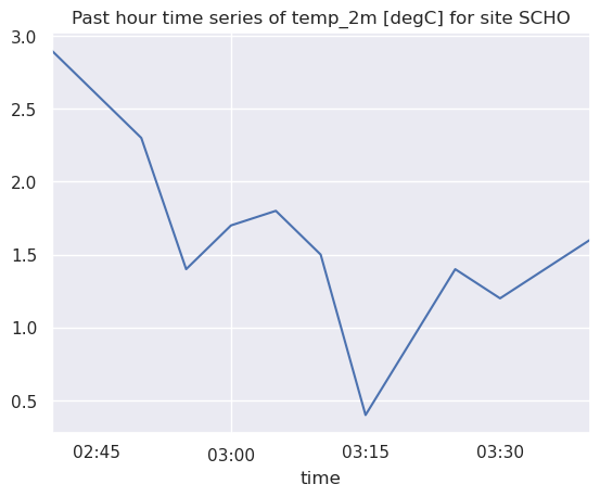
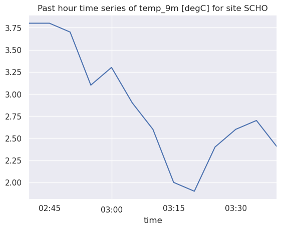
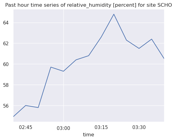
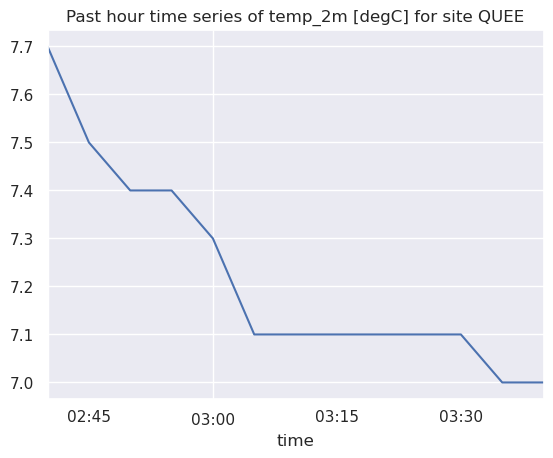
varList = ['temp_2m [degC]', 'temp_9m [degC]', 'relative_humidity [percent]']
# Set your own list of sites here
sites = ['SCHO','QUEE','CHAZ']
Invoke the seaborn library to make our time series plots more readable.
sns.set()
NOTE: To reset the plots to their default look, uncomment and run the following cell. Note how the
seaborn-enabled plots look nicer.#sns.reset_orig()
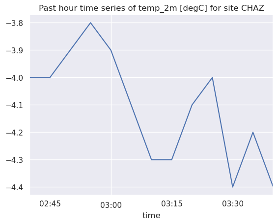
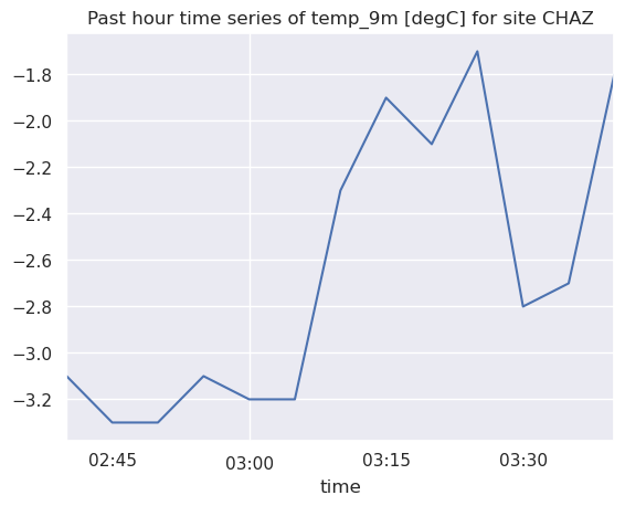
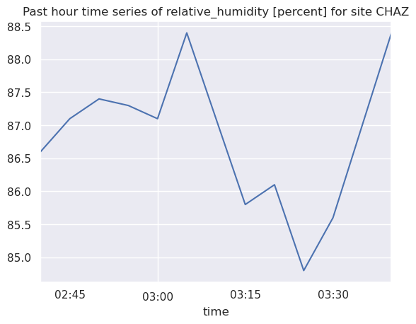
Create a nested for loop over the sites and variables, and make time series plots.
for site in sites:
    for var in varList:
        dfStn = df.query(' station == @site ')
        titleStr = "Past hour time series of " + var + " for site " + site
        dfStn[var].plot(title=titleStr)
        plt.show()

Before you leave ... :
- Save the notebook (File-->Save Notebook)
- Shutdown the notebook (File-->Close and Shutdown Notebook)