02_GriddedDiagnostics_Dewpoint_CFSR: Compute derived quantities using MetPy
Contents
02_GriddedDiagnostics_Dewpoint_CFSR: Compute derived quantities using MetPy
In this notebook, we’ll cover the following:
Select a date and access various CFSR Datasets
Subset the desired Datasets along their dimensions
Calculate and visualize dewpoint.
0) Preliminaries 
import xarray as xr
import pandas as pd
import numpy as np
from datetime import datetime as dt
from metpy.units import units
import metpy.calc as mpcalc
import cartopy.crs as ccrs
import cartopy.feature as cfeature
import matplotlib.pyplot as plt
ERROR 1: PROJ: proj_create_from_database: Open of /knight/anaconda_aug22/envs/aug22_env/share/proj failed
1) Specify a starting and ending date/time, and access several CFSR Datasets
startYear = 2013
startMonth = 5
startDay = 31
startHour = 12
startMinute = 0
startDateTime = dt(startYear,startMonth,startDay, startHour, startMinute)

endYear = 2013
endMonth = 5
endDay = 31
endHour = 18
endMinute = 0
endDateTime = dt(endYear,endMonth,endDay, endHour, endMinute)
Create Xarray Dataset objects
dsZ = xr.open_dataset ('/cfsr/data/%s/g.%s.0p5.anl.nc' % (startYear, startYear))
dsT = xr.open_dataset ('/cfsr/data/%s/t.%s.0p5.anl.nc' % (startYear, startYear))
dsU = xr.open_dataset ('/cfsr/data/%s/u.%s.0p5.anl.nc' % (startYear, startYear))
dsV = xr.open_dataset ('/cfsr/data/%s/v.%s.0p5.anl.nc' % (startYear, startYear))
dsW = xr.open_dataset ('/cfsr/data/%s/w.%s.0p5.anl.nc' % (startYear, startYear))
dsQ = xr.open_dataset ('/cfsr/data/%s/q.%s.0p5.anl.nc' % (startYear, startYear))
dsSLP = xr.open_dataset ('/cfsr/data/%s/pmsl.%s.0p5.anl.nc' % (startYear, startYear))
2) Specify a date/time range, and subset the desired Datasets along their dimensions.
Create a list of date and times based on what we specified for the initial and final times, using Pandas’ date_range function
dateList = pd.date_range(startDateTime, endDateTime,freq="6H")
dateList
DatetimeIndex(['2013-05-31 12:00:00', '2013-05-31 18:00:00'], dtype='datetime64[ns]', freq='6H')
# Areal extent
lonW = -105
lonE = -90
latS = 31
latN = 39
cLat, cLon = (latS + latN)/2, (lonW + lonE)/2
latRange = np.arange(latS,latN+.5,.5) # expand the data range a bit beyond the plot range
lonRange = np.arange(lonW,lonE+.5,.5) # Need to match longitude values to those of the coordinate variable
Specify the pressure level.
# Vertical level specificaton
pLevel = 900
levStr = f'{pLevel}'
We will calculate dewpoint and theta-e, which depend on temperature and specific humidity (and also pressure, as we will see), so read in those arrays. Read in U and V as well if we wish to visualize wind vectors.
Now create objects for our desired DataArrays based on the coordinates we have subsetted.
# Data variable selection
U = dsU['u'].sel(time=dateList,lev=pLevel,lat=latRange,lon=lonRange)
V = dsV['v'].sel(time=dateList,lev=pLevel,lat=latRange,lon=lonRange)
Q = dsQ['q'].sel(time=dateList,lev=pLevel,lat=latRange,lon=lonRange)
T = dsT['t'].sel(time=dateList,lev=pLevel,lat=latRange,lon=lonRange)
Define our subsetted coordinate arrays of lat and lon. Pull them from any of the DataArrays. We’ll need to pass these into the contouring functions later on.
lats = T.lat
lons = T.lon
3) Calculate and visualize dewpoint.
Let’s examine the MetPy diagnostic that calculates dewpoint if specific humidity is available [Dewpoint from specific humidity]:(https://unidata.github.io/MetPy/latest/api/generated/metpy.calc.dewpoint_from_specific_humidity.html)
We can see that this function requires us to pass in arrays of pressure, temperature, and specific humidity. In this case, pressure is constant everywhere, since we are operating on an isobaric surface.
As such, we need to be sure we are attaching units to our previously specified pressure level.
#Attach units to pLevel for use in MetPy with new variable, P:
P = pLevel*units['hPa']
P
Now, we have everything we need to calculate dewpoint.
Td = mpcalc.dewpoint_from_specific_humidity(P, T, Q)
Td
<xarray.DataArray (time: 2, lat: 17, lon: 31)>
<Quantity([[[-0.38378906 -1.5863037   0.24829102 ... 15.448212   16.002563
   16.368134  ]
  [ 0.46426392 -0.78015137 -1.2246399  ... 15.210388   16.000183
   16.526611  ]
  [-0.19406128 -0.55340576 -1.9389954  ... 15.3377075  16.09494
   16.669312  ]
  ...
  [-0.56295776 -4.129303   -4.4381714  ... 17.189545   17.470367
   17.692535  ]
  [ 0.62823486 -1.8757935  -1.2958984  ... 16.632019   17.188995
   17.823822  ]
  [ 5.5015564   1.9374695   0.9364319  ... 16.702728   17.072357
   18.004791  ]]

 [[ 0.27651978 -0.21264648 -0.8648071  ... 17.484436   17.495941
   17.629578  ]
  [-1.8795776  -2.5480042  -3.89859    ... 17.194427   17.21936
   17.609253  ]
  [-4.1887207  -4.072876   -4.8716736  ... 16.726654   16.651093
   17.287903  ]
  ...
  [-5.340027   -7.9271545  -7.942871   ... 17.734283   17.521454
   17.509918  ]
  [-7.479645   -8.929504   -8.049377   ... 17.927765   17.442963
   17.329254  ]
  [-4.255249   -6.4847107  -7.5031433  ... 17.855255   17.41983
   17.134918  ]]], 'degree_Celsius')>
Coordinates:
  * time     (time) datetime64[ns] 2013-05-31T12:00:00 2013-05-31T18:00:00
  * lat      (lat) float32 31.0 31.5 32.0 32.5 33.0 ... 37.0 37.5 38.0 38.5 39.0
  * lon      (lon) float32 -105.0 -104.5 -104.0 -103.5 ... -91.0 -90.5 -90.0
lev float32 900.0Notice the units are in degrees Celsius.
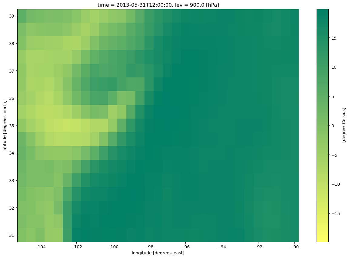
Let’s do a quick visualization.
Td.sel(time=startDateTime).plot(figsize=(15,10),cmap='summer_r')
<matplotlib.collections.QuadMesh at 0x146331cafc40>
Find the min/max values (no scaling necessary). Use these to inform the setting of the contour fill intervals.
minTd = Td.min().values
maxTd = Td.max().values
print (minTd, maxTd)
-11.092773 20.672699
TdInc = 2
TdContours = np.arange (-12, 24, TdInc)
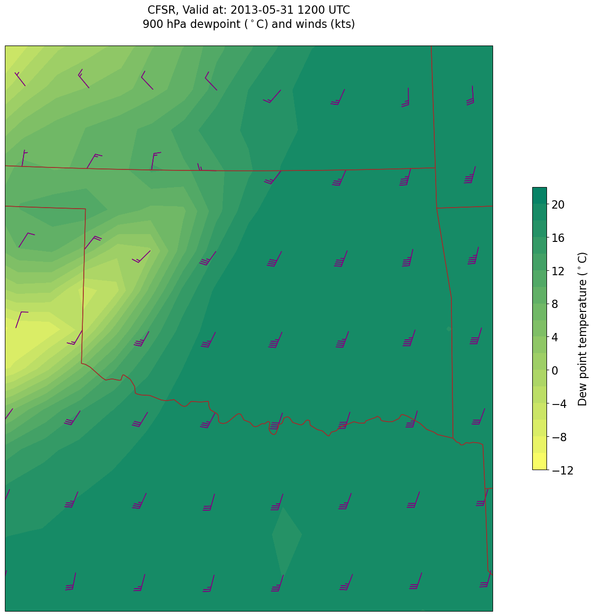
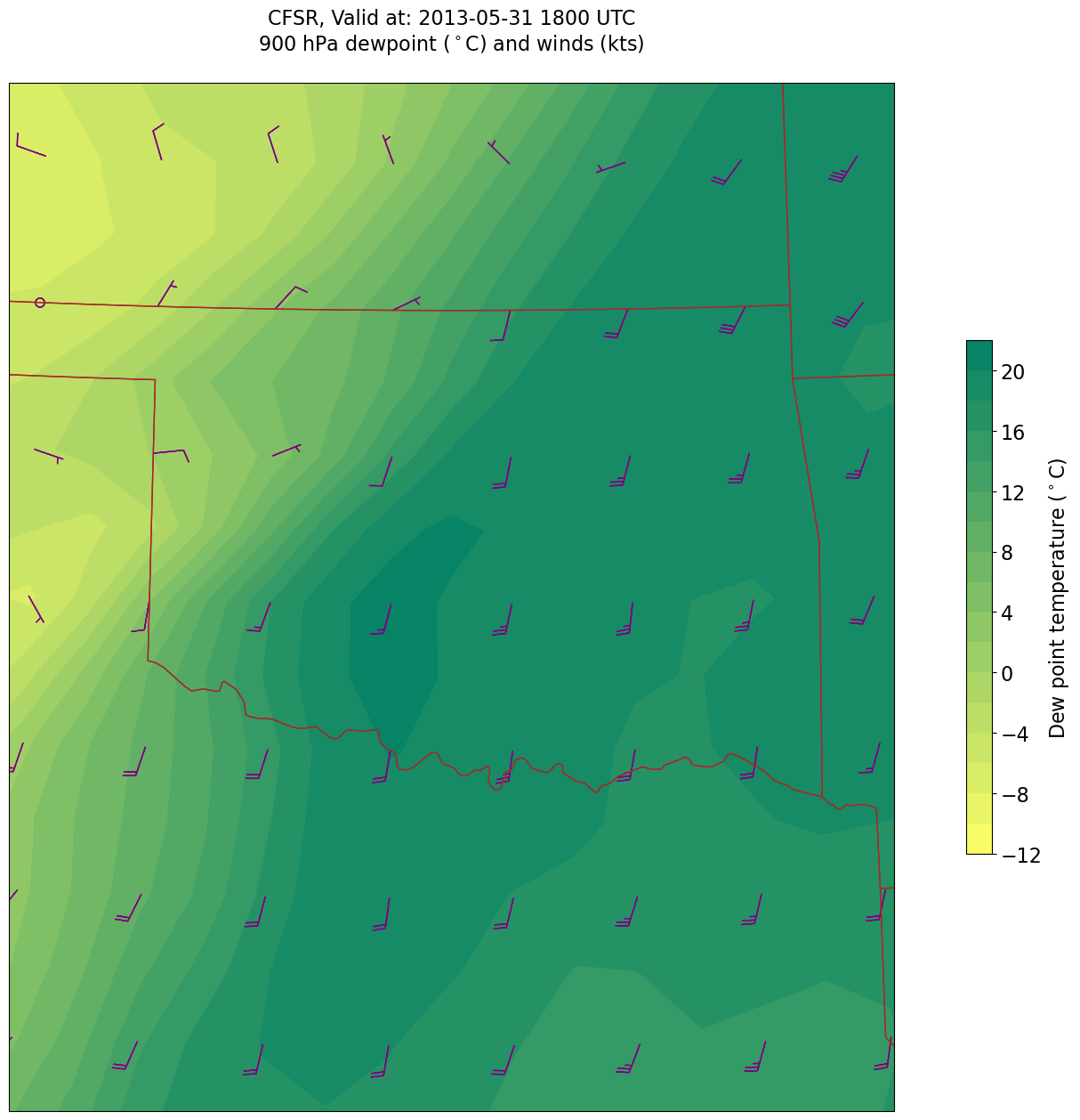
Now, let’s plot filled contours of dewpoint, and wind barbs on the map.
Convert U and V to knots
UKts = U.metpy.convert_units('kts')
VKts = V.metpy.convert_units('kts')
constrainLat, constrainLon = (0.5, 4.0)
proj_map = ccrs.LambertConformal(central_longitude=cLon, central_latitude=cLat)
proj_data = ccrs.PlateCarree() # Our data is lat-lon; thus its native projection is Plate Carree.
res = '50m'
for time in dateList:
    print("Processing", time)

    # Create the time strings, for the figure title as well as for the file name.
    timeStr = dt.strftime(time,format="%Y-%m-%d %H%M UTC")
    timeStrFile = dt.strftime(time,format="%Y%m%d%H")

    tl1 = str('CFSR, Valid at: '+ timeStr)
    tl2 = levStr + " hPa dewpoint ($^\circ$C) and winds (kts)"

    title_line = (tl1 + '\n' + tl2 + '\n')

    fig = plt.figure(figsize=(21,15)) # Increase size to adjust for the constrained lats/lons
    ax = plt.subplot(1,1,1,projection=proj_map)
    ax.set_extent ([lonW+constrainLon,lonE-constrainLon,latS+constrainLat,latN-constrainLat])
    ax.add_feature(cfeature.COASTLINE.with_scale(res))
    ax.add_feature(cfeature.STATES.with_scale(res),edgecolor='brown')

    # Need to use Xarray's sel method here to specify the current time for any DataArray you are plotting.

    # 1. Contour fill of dewpoint.
    cTd = ax.contourf(lons, lats, Td.sel(time=time), levels=TdContours, cmap='summer_r', transform=proj_data)
    cbar = plt.colorbar(cTd,shrink=0.5)
    cbar.ax.tick_params(labelsize=16)
    cbar.ax.set_ylabel("Dew point temperature ($^\circ$C)",fontsize=16)

    # 4. wind barbs
    # Plotting wind barbs uses the ax.barbs method. Here, you can't pass in the DataArray directly; you can only pass in the array's values.
    # Also need to sample (skip) a selected # of points to keep the plot readable.
    # Remember to use Xarray's sel method here as well to specify the current time.
    skip = 2
    ax.barbs(lons[::skip],lats[::skip],UKts.sel(time=time)[::skip,::skip].values, VKts.sel(time=time)[::skip,::skip].values, color='purple',transform=proj_data)

    title = plt.title(title_line,fontsize=16)
    #Generate a string for the file name and save the graphic to your current directory.
    fileName = timeStrFile + '_CFSR_' + levStr + '_Td_Wind.png'
    fig.savefig(fileName)
Processing 2013-05-31 12:00:00
Processing 2013-05-31 18:00:00