THREDDS-served GRIB Data: GFS (Global Grid) Model¶

This notebook reads in realtime GFS model output from a THREDDS server.¶

Overview:¶

Determine latest available model run
Use dictionaries to deal with coordinate dimension names that change from run-to-run
Subset data and map regions
Create a time series of a variable at a point

Imports¶

import cartopy.crs as ccrs
import cartopy.feature as cfeature
from matplotlib import pyplot as plt
from matplotlib.dates import DateFormatter, AutoDateLocator,HourLocator,DayLocator
import numpy as np
import xarray as xr
import pandas as pd
from datetime import datetime, timedelta
from pyproj import Proj
import seaborn as sns
sns.set()

Access real-time NWP data from Unidata’s THREDDS server¶

Parse the current time and choose a recent hour when we might expect the model run to be complete. There is normally a ~90 minute lag, but we’ll give it a bit more than that.

now = datetime.now()
year = now.year
month = now.month
day = now.day
hour = now.hour
minute = now.minute
print (year, month, day, hour,minute)

2023 10 24 23 40

# Allow for a six-hour lag between GFS initialization and current time
if (hour >= 18):
    runHour = 12
    hrDelta = hour - runHour
elif (hour >= 12):
    runHour = 6
    hrDelta = hour - runHour
elif (hour >= 6):
    runHour = 0
    hrDelta = hour - runHour
else:
    runHour = 18
    hrDelta = hour + 6
    
runTime = now - timedelta(hours=hrDelta)
runTimeStr = runTime.strftime('%Y%m%d %H00 UTC')
modelDate = runTime.strftime('%Y%m%d')
modelHour = runTime.strftime('%H')
modelMin = runTime.strftime('%M')
modelDay = runTime.strftime('%D')
titleTime = modelDay + ' ' +  modelHour + '00 UTC'
print (modelDay)
print (modelHour)
print (runTimeStr)
print(titleTime)

10/24/23
12
20231024 1200 UTC
10/24/23 1200 UTC

Open the most recent NCEP real-timeGFS from Unidata’s THREDDS server

ds = xr.open_dataset(f'https://thredds.ucar.edu/thredds/dodsC/grib/NCEP/GFS/Global_0p25deg/GFS_Global_0p25deg_{modelDate}_{modelHour}00.grib2')

Leverage MetPy’s parse_cf function, which among other things will make it easy to extract the dataset’s map projection.

ds = ds.metpy.parse_cf()

Note that there now exists a metpy_crs coordinate variable, which we’ll soon use to determine and use the Dataset’s map projection.

Select one of the variables from the Dataset; in this case, we’ll choose 2-meter temperature.

var = ds.Temperature_height_above_ground

Examine the grid

GRIB files that are served by THREDDS are automatically converted into NetCDF. A quirk in this translation can result in certain dimensions (typically those that are time or vertically-based) varying from run-to-run. For example, the time coordinate dimension for a given variable might be time in one run, but time1 (or time2, time3, etc.) in another run. This poses a challenge any time we want to subset a DataArray. For example, if a particular dataset had vertical levels in units of hPa, the dimension name for the geopotential height grid might be isobaric. If we wanted to select only the 500 and 700 hPa levels, we might write the following line of code:

Z = ds.sel(isobaric=[500, 700])

This would fail if we pointed to model output from a different time, and the vertical coordinate name for geopotential height was instead isobaric1.

Via strategic use of Python dictionaries, we can programmatically deal with this!

First, let’s use some MetPy accessors that determine the dimension names for times and vertical levels:

timeDim, vertDim = var.metpy.time.name, var.metpy.vertical.name
timeDim, vertDim

('time1', 'height_above_ground3')

We next construct dictionaries corresponding to each desired subset of the relevant dimensions. Here, we specify the first time, and the one and only vertical level:

idxTime = 0 # First time
idxVert = 0 # First (and in this case, only) vertical level

timeDict = {timeDim: idxTime}
vertDict = {vertDim: idxVert}

timeDict, vertDict

({'time1': 0}, {'height_above_ground3': 0})

Produce a quick visualization at the given time and level. Pass the two dictionaries into Xarray’s isel function.

grid = var.isel(timeDict).isel(vertDict)
grid.plot()

<matplotlib.collections.QuadMesh at 0x14b76d45f690>

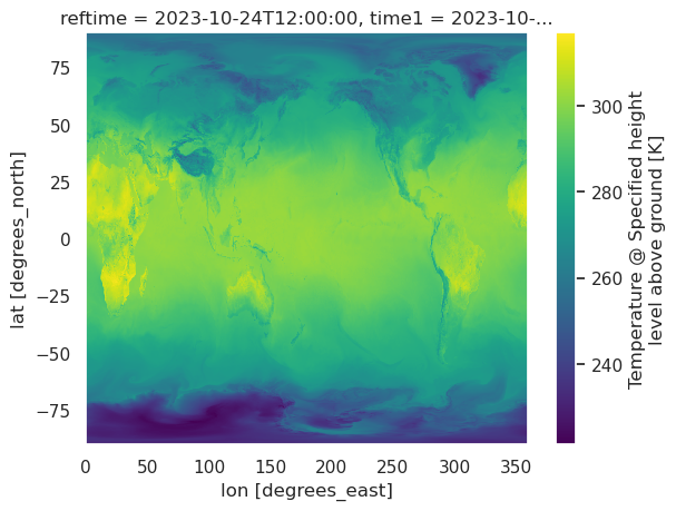
../../_images/9b2b5efffdae40b9896455d12bfd8b2feaafb22c4c7bf9e2ab3b2a836e25c62d.png

Get the Dataset’s map projection.

proj_data = var.metpy.cartopy_crs
proj_data

<cartopy.crs.PlateCarree object at 0x14b6f018d1d0>

Plot the data over the full domain

Create a title string

validTime = var.isel(timeDict)[timeDim].values # Returns validTime as a NumPy Datetime 64 object
validTime = pd.Timestamp(validTime) # Converts validTime to a Pandas Timestamp object
timeStr = validTime.strftime("%Y-%m-%d %H%M UTC") # We can now use Datetime's strftime method to create a time string.
tl1 = "GFS 2m temperature ($^\circ$C)"
tl2 = str('Valid at: '+ timeStr)
title_line = (tl1 + '\n' + tl2 + '\n')

Convert grid to desired units

grid = grid.metpy.convert_units('degC')

Create DataArray objects for the horizontal coordinate dimensions. In this case, the model is output on global cylindrical equidistant (PlateCarree) projection, which means the horizontal dimensions are named lon and lat and represent grid point locations in degrees.

x, y = ds.lon, ds.lat

res = '110m'
fig = plt.figure(figsize=(18,12))
ax = plt.subplot(1,1,1,projection=proj_data)

ax.set_facecolor(cfeature.COLORS['water'])
ax.add_feature (cfeature.LAND.with_scale(res))
ax.add_feature(cfeature.COASTLINE.with_scale(res))
ax.add_feature (cfeature.LAKES.with_scale(res), alpha = 0.5, zorder=4)
ax.add_feature (cfeature.STATES.with_scale(res))
# Usually avoid plotting counties once the regional extent is large
#ax.add_feature(USCOUNTIES,edgecolor='grey', linewidth=1 );
CF = ax.contourf(x,y,grid,cmap='coolwarm',alpha=0.99,transform=proj_data)
cbar = plt.colorbar(CF,fraction=0.046, pad=0.03,shrink=0.5)
cbar.ax.tick_params(labelsize=10)
cbar.ax.set_ylabel(f'Temperature ($^\circ$C)',fontsize=10);
title = ax.set_title(title_line,fontsize=16)

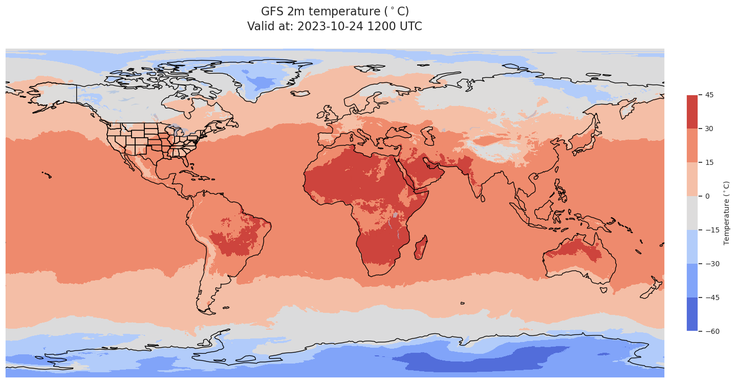
../../_images/ce7107acfa1edb4d16d80f31c5aee082236dfc393e0cc01358b46979caefa8fc.png

Subset the dataset to a smaller region¶

The longitudes range from 0 to 359.75 degrees East. For the purposes of selecting ranges which include points in the western hemisphere, express these values as positive numbers. The latitudes go from north to south … i.e., in decreasing order.

lonW, lonE, latS, latN = [-80 + 360, -71+360, 40, 45]
mapExtent = lonW, lonE, latS, latN

We can directly select latitude and longitude values to perform regional subset selections; no need to use the Pyproj library.¶

Determine the grid spacing

delX, delY = ( (x[1] - x[0]), (y[1] - y[0]) )

In order for the data region to fill the plotted region, pad the longitude and latitude ranges (trial and error, depends on the subregion)

xPad = 4
yPad = 4

xRange = np.arange(lonW - xPad, lonE + xPad, delX)
yRange = np.arange(latN + yPad, latS - yPad, delY)

Read in the temperature data over the selected region. Also subset the time and vertical coordinates. Convert the units.

dsSub = ds.sel(lon = xRange, lat = yRange)
xSub, ySub = dsSub.lon, dsSub.lat
varSub = dsSub.Temperature_height_above_ground
gridSub = varSub.isel(timeDict).isel(vertDict)
gridSub = gridSub.metpy.convert_units('degC')

Specify the output map projection (Lambert Conformal, centered on New York State)

lon1 = -75
lat1 = 42.5
slat = 42.5

proj_map= ccrs.LambertConformal(central_longitude=lon1,
                             central_latitude=lat1,
                             standard_parallels=[slat,slat])

Plot the regional map. Omit plotting the land/water features since they tend to obscure the nuances of the temperature field. This also speeds up the creation of the figure.

res = '10m'
fig = plt.figure(figsize=(18,12))
ax = plt.subplot(1,1,1,projection=proj_map)
ax.set_extent(mapExtent, crs=ccrs.PlateCarree())
#ax.set_facecolor(cfeature.COLORS['water'])
#ax.add_feature (cfeature.LAND.with_scale(res))
ax.add_feature(cfeature.COASTLINE.with_scale(res))
#ax.add_feature (cfeature.LAKES.with_scale(res), alpha = 0.5)
ax.add_feature (cfeature.STATES.with_scale(res))
# Usually avoid plotting counties once the regional extent is large
#ax.add_feature(USCOUNTIES,edgecolor='grey', linewidth=1 );
CF = ax.contourf(xSub,ySub,gridSub, cmap='coolwarm',alpha=0.5,transform=proj_data)
cbar = plt.colorbar(CF,fraction=0.046, pad=0.03,shrink=0.5)
cbar.ax.tick_params(labelsize=10)
cbar.ax.set_ylabel(f'Temperature ($^\circ$C)',fontsize=10);
title = ax.set_title(title_line,fontsize=16)

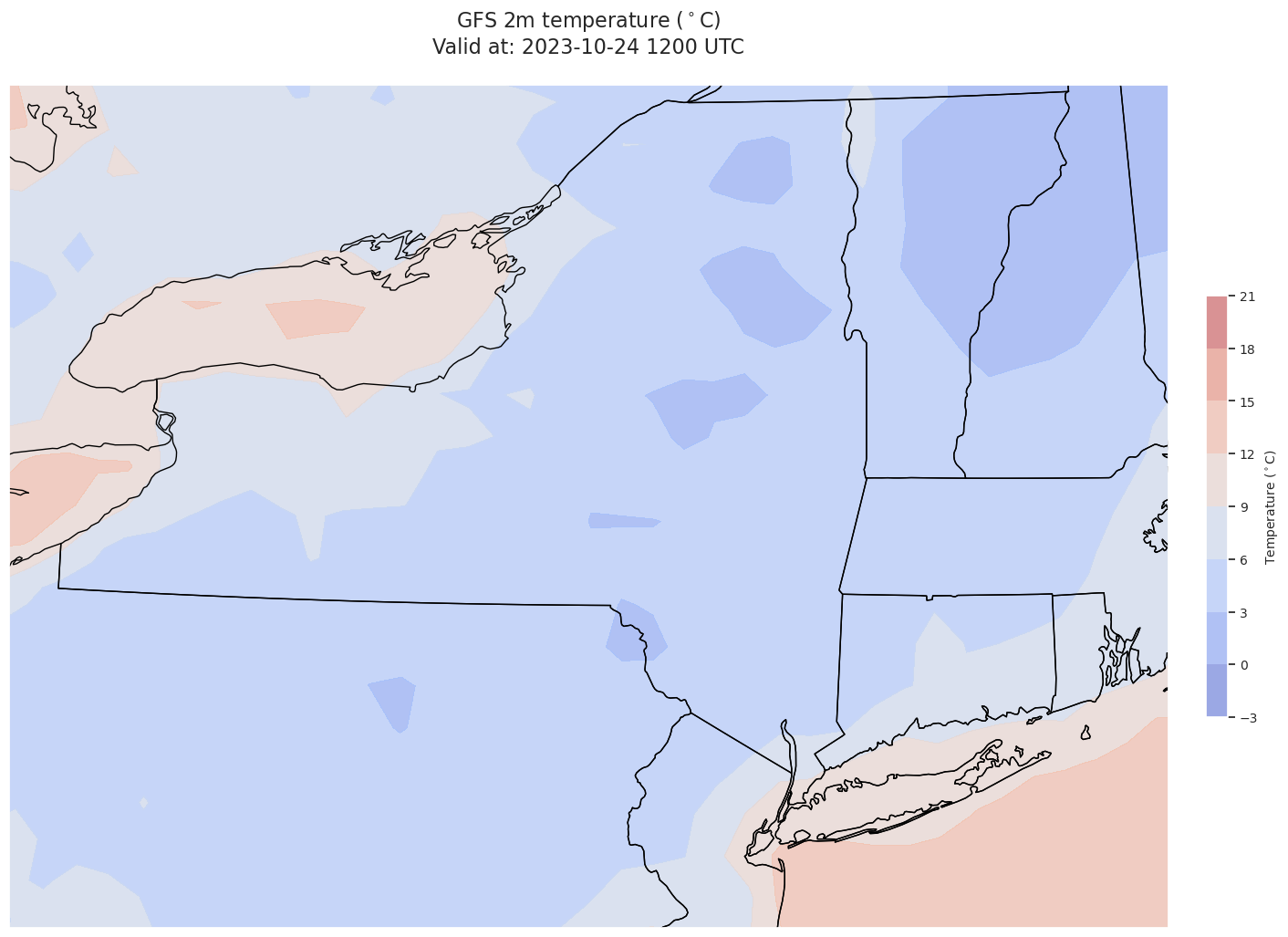
../../_images/fa2154fc77755ef814d9bed65733acb8d18f4e9ecb8a244658d356364c7fdbd8.png

Create a time series at the gridpoint closest to a given location.¶

siteName = "ALB"
siteLat, siteLon = (42.75, -73.8 + 360) # ALB Airport; pay attention to whether western hemipshere longitudes are expressed as negative or positive

Subset the full grid, and convert the units. For the time series, we want all times, so we don’t subset the time dimension.

timeSer = var.sel(lon = siteLon, lat = siteLat, method='nearest').isel(vertDict)
timeSer = timeSer.metpy.convert_units('degC')
times = timeSer[timeDim]

fig = plt.figure(figsize=(15,10))
fig.suptitle(f'GFS {validTime} Initialization',fontweight='bold',fontsize=15)
ax = fig.add_subplot(111)

ax.set_xlabel('Date/Time')
ax.set_ylabel('2 m Temperature ($^\circ$C)')
ax.set_title(f'Time series at gridpoint closest to {siteName}: Latitude {siteLat} , Longitude {siteLon}' )


# Improve on the default ticking

ax.plot(times, timeSer, linewidth=0.8,color='tab:blue',marker='o',linestyle='--')
ax.xaxis.set_major_locator(HourLocator(interval=12)) # Select an appropriate interval based on the dataset
hoursFmt = DateFormatter('%d/%H')

ax.xaxis.set_major_formatter(hoursFmt)
ax.tick_params(axis='x', rotation=45, labelsize=8)
ax.set_xlim(times.values[0],times.values[-1]);                                         

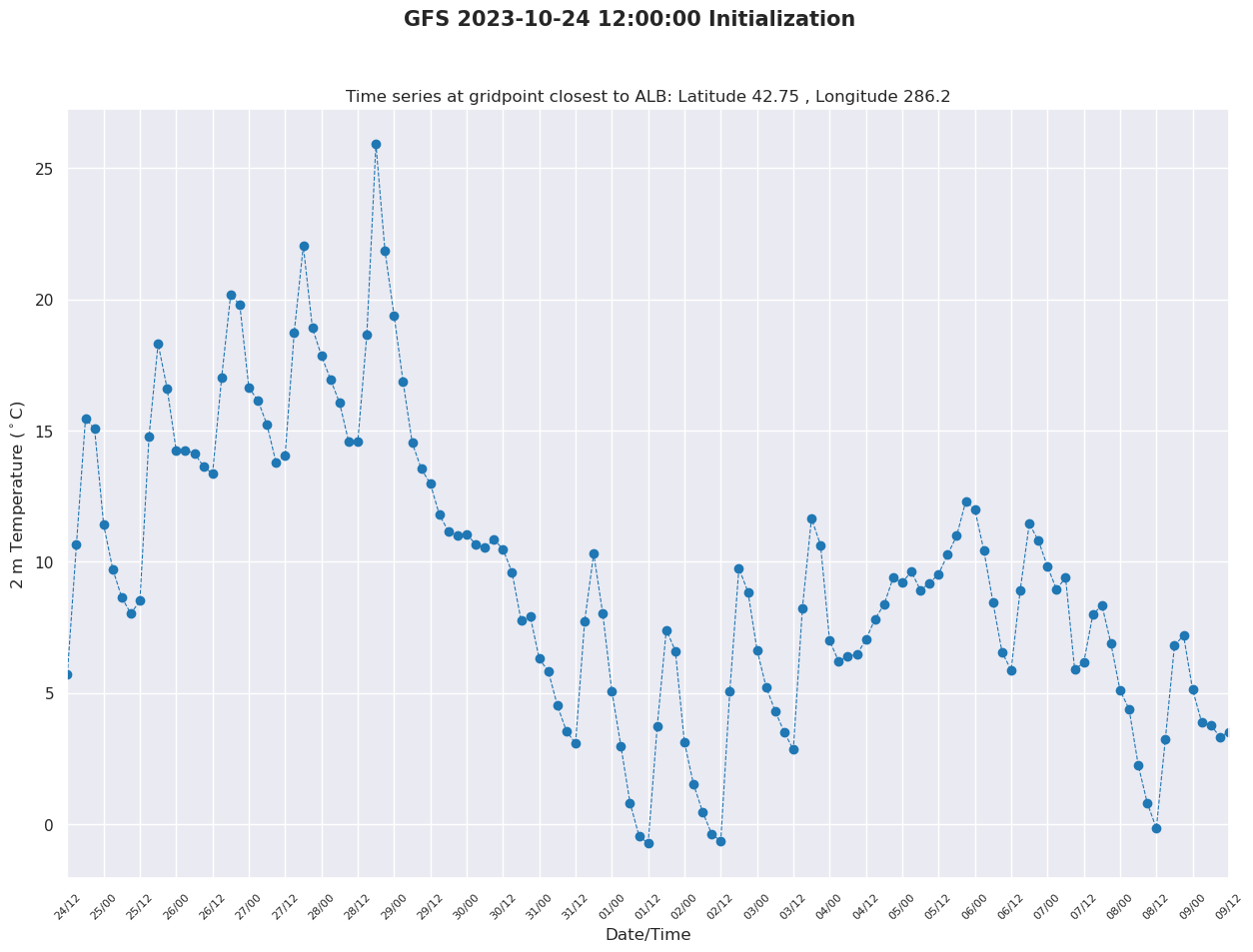
../../_images/e6cb8115cf179cacc9bc66e72fd6d79bed371b01b9242c1ba6f9dcbaf43c6ad8.png

Things to try:¶

Try other variables, locations, and global models
Create a suite of forecast products, looping over forecast hours, model levels, etc.

ATM433/533 Fall 2023

THREDDS-served GRIB Data: GFS (Global Grid) Model

Contents