04_Geoviews_Datashader_NLDN
Contents
04_Geoviews_Datashader_NLDN
Overview:
Read in a multi-million row dataframe containing National Lightning Detection Network data from August 2021
Use
Datashaderto create a rasterized representation of the dataframeCreate an interactive, georeferenced visualization of NLDN data using the Holoviz ecosystem
Prerequisites
Concepts |
Importance |
Notes |
|---|---|---|
Pandas |
Necessary |
|
Geoviews 1-2 |
Necessary |
Time to learn: 30 minutes
Imports
import datashader as ds
import pandas as pd
from colorcet import fire
from datashader import transfer_functions as tf
import geoviews as gv
from geoviews import opts
import holoviews as hv
from holoviews.element.tiles import OSM
from holoviews.operation.datashader import datashade,rasterize
hv.extension('bokeh')


Read in a multi-million row dataframe containing National Lightning Detection Network data from August 2021
Here, we load in all of the detected cloud-to-ground flashes from August 2021. The data was originally derived from a Pandas-friendly text file, with over 50 million lines (one per flash, cloud-to-cloud as well as cloud-to-ground). While we could use Pandas read_csv to create a Dataframe from it, here we read in the dataset as expressed in Feather format.
%time df = pd.read_feather('/spare11/atm533/data/202108_NLDN_CG.ftr')
CPU times: user 456 ms, sys: 394 ms, total: 850 ms
Wall time: 389 ms
df
| Lat | Lon | Cur | CG | DateTime | |
|---|---|---|---|---|---|
| 0 | 39.9854 | -108.4006 | -13.0 | G | 2021-08-01 00:00:00.020462336 |
| 1 | 37.3190 | -94.6979 | -14.0 | G | 2021-08-01 00:00:00.166759424 |
| 2 | 37.3117 | -94.6988 | -18.7 | G | 2021-08-01 00:00:00.214292480 |
| 3 | 37.3001 | -94.7059 | -15.9 | G | 2021-08-01 00:00:00.278298624 |
| 4 | 33.2999 | -102.8773 | -29.8 | G | 2021-08-01 00:00:00.343449600 |
| ... | ... | ... | ... | ... | ... |
| 10442992 | 34.2253 | -110.5720 | -12.2 | G | 2021-08-31 23:59:58.720049920 |
| 10442993 | 38.7619 | -90.9445 | -7.5 | G | 2021-08-31 23:59:58.799020800 |
| 10442994 | 34.2261 | -110.5723 | -6.1 | G | 2021-08-31 23:59:58.917163264 |
| 10442995 | 34.2251 | -110.5716 | -13.4 | G | 2021-08-31 23:59:59.009214720 |
| 10442996 | 33.7232 | -115.8189 | 35.1 | G | 2021-08-31 23:59:59.471597056 |
10442997 rows × 5 columns
Plot flash locations using Pandas’ Matplotlib Scatterplot interface.
df.plot.scatter('Lon','Lat',figsize=(11,8));
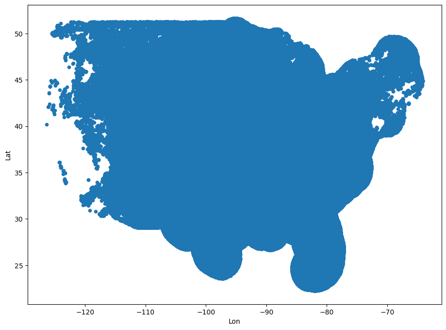
The plot takes a while to appear, and is essentially useless due to the thousands upon thousands of overlapping points. It seems impossible to make a useful plot of a month’s worth (tens of millions of flashes during the warm season) of lightning strikes … until we leverage the Datashader library, which is part of Holoviz.
Use Datashader to create a rasterized representation of the dataframe
First, we will directly use Datashader methods to produce a visualization. We set up a Datashader Canvas object of x by y pixels, and then aggregate each point into a raster image of the specified x by y dimensions.
Then, we use Datashader’s transfer_functions methods to set a colormap and a background.
agg = ds.Canvas(800,600).points(df,'Lon','Lat')
tf.set_background(tf.shade(agg, cmap=fire),"black")

What previously took a minute or so and provided only the coarsest amount of detail, now takes place in seconds and the detail is such that we can clearly see the implied geography!
However, as cool (or, in the case of this colormap, hot) as the above graphic is, it has no interactivity nor georeferencing (technically, a Datashader object has no concept of things like axes or colorbars.
Holoviews and Geoviews to the rescue!
Create an interactive, georeferenced visualization of NLDN data using the Holoviz ecosystem
First, create a Geoviews dataset from the Pandas dataframe
gdf = gv.Dataset(df)
Now, we create two Geoviews objects; one for a background map, and the other, NLDN flash locations derived from GeoViews’ representation of the underlying Dataframe.
map_tiles  = OSM().opts(alpha=0.9,width=900, height=700)
points     = gv.Points(gdf, ['Lon','Lat'])
Rasterize (and datashade) the points.
flashes = rasterize(points, x_sampling=.001, y_sampling=.001, cmap=fire, alpha=100)
- x_ and y_sampling specify to what resolution the points should be sampled from, using the distance coordinates relevant to the dataset. Here, we specify to sample every thousandth of a degree.
- We specify the
alphaargument as a value from 0 to 255 here, as opposed to a floating point range of 0 to 1. This will make it so we can see the underlying map background.
Add in some options
We’ll add a colorbar, a log scale, and the hover tool.
flashes = flashes.opts(colorbar=True,logz=True,width=900,height=700,tools=['hover'])
Create the final graphic
Overlay the rasterized flashes with the OpenStreetMaps background
flashmap = map_tiles * flashes
View and interact with the map
flashmap
Notice how quickly the map updates! The rasterized image’s detail changes with zoom just as you are used to with other web-based mapping tools, such as Google Maps!
Examine the Pandas dataframe: subset latitude and longitude so you can determine when these strikes occurred.
Summary
We have successfully and efficiently loaded, visualized, and interacted with a very large dataset!
Nevertheless, the memory footprint remains large enough so that it is not practical to have several users working with this dataset simultaneously.