Class Summaries
Th 24 Jan
- Time Magazine’s Famous Cover Story on Carl Gustav Rossby from 17 December 1956 (PDF)
- A Reality Check on Federal Entitlement and Discretionary Spending (PPTX)
- Discussed the meteorological job state of the union, where generic weather forecasting positions are becoming more and more limited as added skills in addition to basic meteorological knowledge become more important to employers.
- Stressed the importance of having both technical skills/software smarts and meteorological knowledge, having something of value to add to a job, and having good writing and speaking skills in order to stay competitive in the meteorological job market.
- Discussed new international city forecast game and map discussion procedure.
- SPC Forecasting Tools (Link)
- Contains:
Upper-Air Maps
Observed Sounding Analysis
Sounding Climatology
Mesoscale Graphics
High Resolution Rapid Refresh Model (HRRR)
High Resolution Ensemble Forecast version 2 (HREFv2)
Short-Range Ensemble Forecast (SREF)
Short-Range Ensemble Plumes
Fire Weather Composite Maps
CompMap
- Contains:
- ECMWF Newsletters (Link)
- Climate Prediction Center (Link)
- Topographic Maps (Link)
Tu 29 Jan
Brief recap of the Dec 1956 Time Magazine story on Carl Gustav Rossby:
- Rossby phase speed and group velocity derivations (Shortcut to Protected Files)
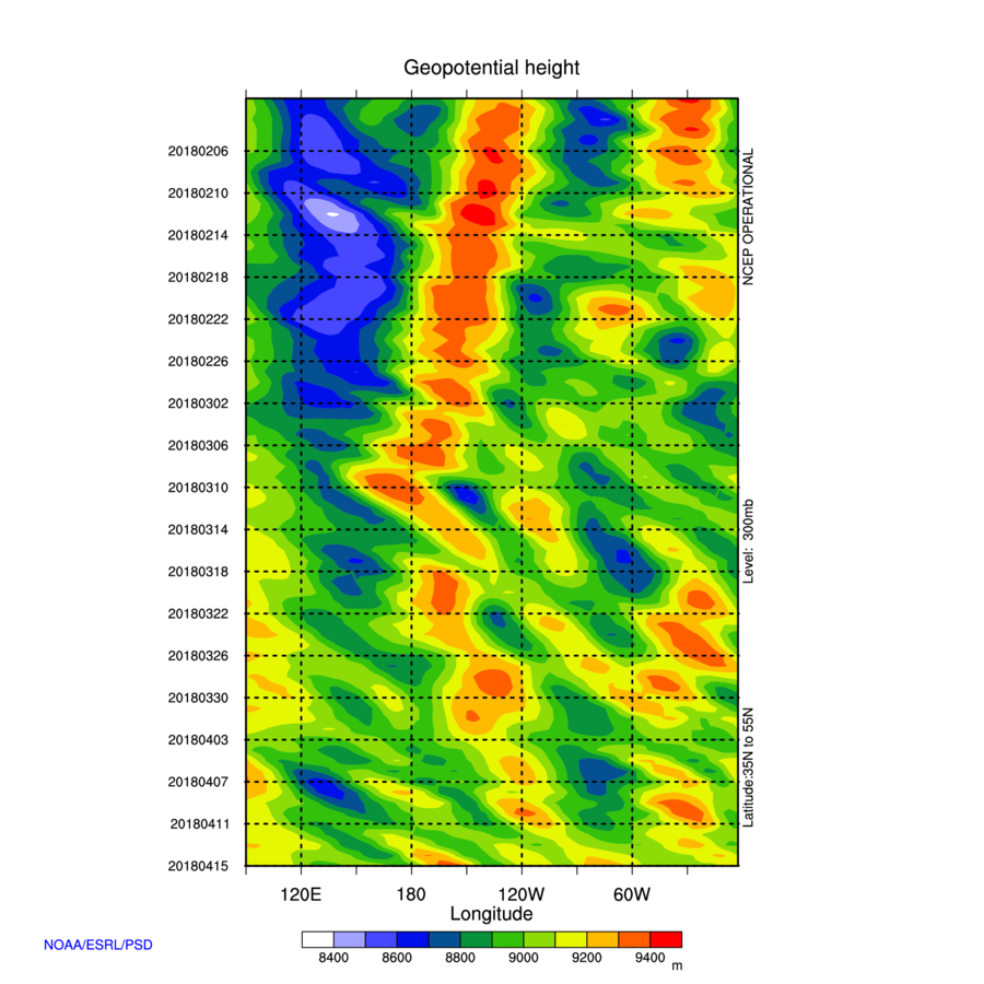
- Hovmoeller 300-hPa mean geopotential heights for 1 Feb to 15 Apr 2018 (PNG)
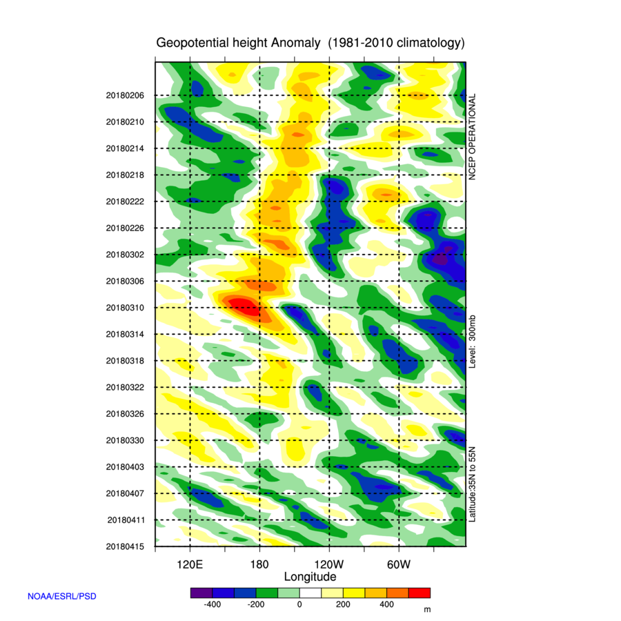
- Hovmoeller 300-hPa anomaly geopotential heights for 1 Feb to 15 Apr 2018 (PNG)
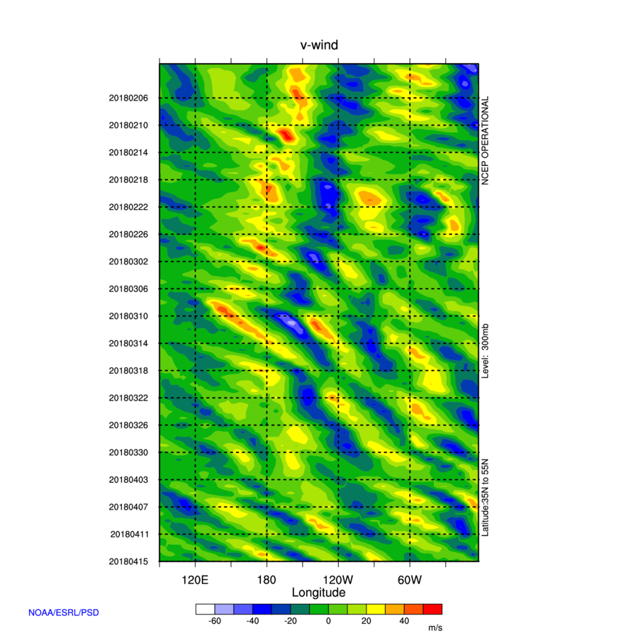
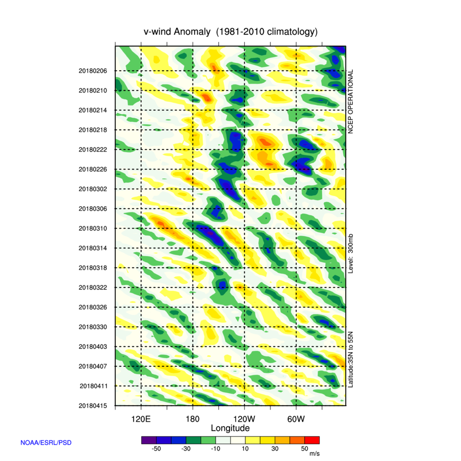
- Hovmoeller 300-hPa mean meridional (v) winds for 1 Feb to 15 Apr 2018 (PNG)
- Hovmoeller 300-hPa anomaly meridional (v) winds for 1 Feb to 15 Apr 2018 (PNG)
First International Forecast Discussion:
a) Work together as two teams (undergrads and grads) before class to produce the forecast products described below.
b) Undergrad team leads on Tuesday; grad team leads on Thursday.
c) Each team should create an AFD before the start of class at 4:15 pm and send it to Marshall Pfahler for posting.
d) Decide how to partition your AFD discussion: One possibility: 1) student A presents the big picture, and 2) student B discusses days 7–10, 4–6, and 1–3. Feel free to choose other possibilities.
e) Make probabilistic temperature and rainfall forecasts for the two initial 3-day periods and the one final 4-day period. Determine: (1) the expected 10th, 50th (over-under number), and 90th percentiles for maximum and minimum temperature during each of the three periods, and (2) the expected 10th, 50th (over-under number) and 90th precipitation amount percentiles during each of the three periods (it’s possible that your precipitation amount percentiles will all be zero if you are expecting dry weather during each of the three periods).
f) To be determined how practical item e) will be. Try it. If to doesn’t work, we’ll modify the plan.
g) Work with Marshall Pfahler to post your probabilistic forecasts to the class home page.
Climatological Information:
- Reykjavik (Link)
- Barcelona (Link)
Learning Experience:
Accept that you will stumble and bumble your way through the probabilistic forecasting process initially. Things will be chaotic on day 1 and likely still chaotic on day 2. You will no doubt want to kill me. It will take you several classes to get things right. Be innovative. Take chances. Think outside the box.
Th 31 Jan
How innovative science thrives: The story of Bell Labs:
- True Innovation: NYT 25 Feb 2012 (Link)
- Why Bell Labs was so Important to Innovation in the 20th Century (Link)
- History of Bell Labs (Link)
- Bell Labs -- Wikipedia (Link)
Automation and the future:
- 27 Jan 2019 New York Times: The Hidden Automation Agenda of the Davos Elite (Link)
Bosart (2003): Whither the Weather Analysis and Forecasting Process (PDF)
Tu 5 Feb
Bosart (2003): Whither the Weather Analysis and Forecasting Process (PDF)
Discussion of the many scientific and operational contributions of Jerome (Jerry) Namias to sub-seasonal and seasonal predictability:
- Namais picture (Link)
- MIT Namias biography (Link)
- Namias biography (John Roads) (Link)
- The Bulletin interviews Jerome Namias. WMO Bulletin, 37, No. 3, July 1988 (Link)
- The Namias Symposium (published 1 Aug 1986) (Link)
- Lance's post to maplist from 19 March 2010 (PDF)
- Galarneau & Bosart (2006): Ridge Rollers: Mesoscale Disturbances on the Periphery of Cutoff Anticyclones (PDF)
Th 7 Feb
Ted Fujita:
- Ted Fujita bio (Link)
- Fujita (1955): Results of Detailed Synoptic Studies of Squall Lines (PDF)
Tu 12 Feb
Discussion of the many scientific and operational contributions of Jerome (Jerry) Namias to sub-seasonal and seasonal predictability:
- Namais picture (Link)
- MIT Namias biography (Link)
- National Academy of Sciences Biographical Jerome Namias Memoir (John Roads) (Link)
- The Bulletin interviews Jerome Namias. WMO Bulletin, 37, No. 3, July 1988 (Link)
- The Namias Symposium (published 1 Aug 1986) (Link)
- Lance's post to maplist from 19 March 2010 (PDF)
- Galarneau & Bosart (2006): Ridge Rollers: Mesoscale Disturbances on the Periphery of Cutoff Anticyclones (PDF)
Discussion of the Blizzard of ’78:
- The Blizzard of ’78 Revisited (courtesy of NWS-Norton) (Link)
- Looking back at the Blizzard of ’78 (Link)
Th 14 Feb
Discussion of the sting jet:
Schultz, D. M. and Browning, K. A. (2017): What is a sting jet? (PDF)
- Highlights from Schultz and Browning (2017): What is a Sting Jet?
- Figure 2: Conceptual model for sting jet location from Schultz and Browning (2017):
a) Sting jets occur near the end of the bent-back occluded front in a region of lower-level frontolysis and close to the tip of the cloud head
b) Sting jets represent a mesoscale wind maximum associated with midtropospheric descent along the bent-back occluded front.
c) Sting jet and cold conveyor belt low-level jet are distinct and separate features and occur to the west of the warm conveyor belt low-level jet.
- Physical mechanisms that have been proposed to explain sting jet origin:
a) Sting jet air originates in weak flow between 850-650-hPa, descends to near the surface in conjunction with strong cold-air advection, and accelerates in an area of a strengthening horizontal pressure gradient.
b) Descending air from the middle troposphere (600-400 hPa) brings down higher momentum air from aloft.
c) Descending air parcels accelerate downward due to evaporative cooling in the lower troposphere which reduces the static stability and enables higher momentum air to reach the surface analogous to convectively driven downdrafts.
d) Surface heat fluxes over oceanic regions can further reduce lower tropospheric static stability and facilitate the downward transport of higher momentum air.
e) Location of the surface wind maximum downstream of the region of the strongest SLP gradient argues for the importance of isallobaric effects and an associated along-flow pressure gradient in accelerating the surface winds.
- Sting Jet in 4 Jan 2018 North Atlantic Bomb Cyclone
- Jom Steenburgh’s post to map about associated sting jet (PDF)
- Heather Archambault loops (Link)
- Possible Continental Sting Jet Case: The Groundhog Day Gale of 2 February 1976
- February Record Low Sea Level Pressures through 2014 (David Roth):
- Link 1
- Link 2
- Bangor, Maine, Historic Flood of 2 February 1976
- Weather Underground History Archive: Selected Station Reports for 1 February 1976:
- ALB
- BDL
- BOS
- PWN
- CON
- BGR
Discussion of the Shapiro-Keyser cyclone model:
- James Steenburgh: Shapiro-Keyser Frontal Cyclone Model (Link)
Tu 19 Feb
The Presidents’ Day storm of 19 Feb 1979 revisited on the occasion of its 40 the anniversary with special guest Dr. Louis Uccellini, Director, National Weather Service and NOAA Assistant Administrator for Weather Services:
- Presidents' Day 1979 page (Link)
Th 21 Feb
- Presidents' Day 1979 page (Link)
- Bosart (1981): The Presidents' Day Snowstorm of 1819 February 1979: A Subsynoptic-Scale Event (PDF)
- Selected ERA5 plots (Tomer Burg) (Link)
Tu 26 Feb
- HW #3 announced (Presidents’ Day II storm of 16–17 Feb 2003):
- Southern Stream Storm 11–17 February 2003: Presidents Day Weekend Snow Storm: Richard Grumm
- NH mean and anomaly maps before and after the Presidents’ Day II storm of 16–17 Feb 2003: NOAA/ESRL
- CFSR Loops: Alicia Bentley
- Selected ERA5 plots (Tomer Burg) (Link)
- Discussion of recent ECMWF newsletters:
- Winter 2018–2019 (Link)
- A new product to flag up the risk of cold spells in Europe weeks ahead (Link) - Autumn 2018 (Link)
- Roberto Buzz talks about probabilistic forecasting and life after ECMWF (Link) - Summer 2018 (Link)
- ECMWF Forecast User Guide (Link) - Spring 2018 (Link)
- Promising results for lightning prediction (Link) - Winter 2017–2018 (Link)
- Autumn 2017 (Link)
- Summer 2017 (Link)
- Spring 2017 (Link)
- Winter 2016–2017 (Link)
- Winter 2018–2019 (Link)
- The ECMWF Ensemble Prediction System (PDF)
Th 28 Feb
- ECMWF Newsletters (Link)
- Discussion of recent ECMWF newsletters:
- Winter 2018–2019 (Link)
- A new product to flag up the risk of cold spells in Europe weeks ahead (Link) - Autumn 2018 (Link)
- Roberto Buzz talks about probabilistic forecasting and life after ECMWF (Link) - Summer 2018 (Link)
- ECMWF Forecast User Guide (Link) - Spring 2018 (Link)
- Promising results for lightning prediction (Link) - Winter 2017–2018 (Link)
- Autumn 2017 (Link)
- Summer 2017 (Link)
- Spring 2017 (Link)
- Winter 2016–2017 (Link)
- Winter 2018–2019 (Link)
- The ECMWF Ensemble Prediction System (PDF)
Tu 5 Mar
- Metric Scales (Link)
- ECMWF Newsletters (Link)
- Discussion of recent ECMWF newsletters:
- Winter 2018–2019: Cold spells in Europe (pp. 15–20) (Link)
- Autumn 2018: European heat wave (pp. 2–3); Aeolus wind date (p. 9), Radiosonde descent data (p. 10), Ship roads (pp. 11–12); Roberto Buzz (pp. 18–19) (Link)
- Summer 2018: Ocean coupling effects (pp. 6–7); Ensemble vertical profiles (pp. 37–42) (Link)
- Spring 2018: El Nino Pacific heat budgets for 1995–1996 vs. 2015–2016 (pp. 4–5); Lightning predictions (pp. 14–19) (Link)
- Winter 2017–2018 Why warm conveyor belts matter in NWP (pp. 21–28)(Link)
- Summer 2017: 10 years of forecasting atmospheric composition at ECMWF (pp. 5–6) (Link)
- Spring 2017: 25 years of ensemble forecasting at ECMWF (pp. 20–31) (Link)
- Winter 2018–2019: Cold spells in Europe (pp. 15–20) (Link)
Th 7 Mar
- ECMWF Newsletters (Link)
- Discussion of recent ECMWF newsletters:
- Autumn 2018: European heat wave (pp. 2–3); Aeolus wind date (p. 9), Radiosonde descent data (p. 10), Ship roads (pp. 11–12); Roberto Buzz (pp. 18–19) (Link)
- Summer 2018: Ocean coupling effects (pp. 6–7); Ensemble vertical profiles (pp. 37–42) (Link)
- Spring 2018: El Nino Pacific heat budgets for 1995–1996 vs. 2015–2016 (pp. 4–5); Lightning predictions (pp. 14–19) (Link)
- Autumn 2018: European heat wave (pp. 2–3); Aeolus wind date (p. 9), Radiosonde descent data (p. 10), Ship roads (pp. 11–12); Roberto Buzz (pp. 18–19) (Link)
Tu 12 Mar
- Exam #1
Th 14 Mar
- Overview of Exam #1
- Discussion Hovmoeller diagrams & downstream development:
- Bosart et al. (2017): Interactions of North Pacific Tropical, Midlatitude, and Polar Disturbances Resulting in Linked Extreme Weather Events over North America in October 2007 (Link)
- THORPEX: The Observing System Research and Predictability Experiment (WMO) (Link)
- Orlanski and Sheldon (1995): Stages in the energetics of baroclinic systems (PDF)
- Discussion of recent ECMWF newsletters:
- The ECMWF Ensemble Prediction System (PDF)
Tu 26 Mar
- Cruise Ship vs. Intense Cyclone:
- World Clock (Link)
- Kepler’s Laws of Planetary Motion (Link)
- Discussion of recent ECMWF newsletters:
- The ECMWF Ensemble Prediction System (PDF)
- Palmer and Richardson (2014): Decisions, decisions….! (from ECMWF Autumn 2014 Newsletter) (Link)
- Buizza et al. (2015): Living with the Butterfly Effect: A Seamless View of Predictability (from ECMWF Autumn 2015 Newsletter) (Link)
- Buizza and Richardson (2017): 25 Years of Ensemble forecasting at ECMWF (from ECMWF Autumn 2017 Newsletter) (Link)
- Palmer (2017): The Primacy of Doubt (PDF)
Th 28 Mar
- ECMWF Forecast User Guide:
- The ECMWF Ensemble Prediction System (PDF)
- Palmer and Richardson (2014): Decisions, decisions….! (from ECMWF Autumn 2014 Newsletter) (Link)
- Buizza et al. (2015): Living with the Butterfly Effect: A Seamless View of Predictability (from ECMWF Autumn 2015 Newsletter) (Link)
- Buizza and Richardson (2017): 25 Years of Ensemble forecasting at ECMWF (from ECMWF Autumn 2017 Newsletter) (Link)
- Palmer (2017): The Primacy of Doubt (PDF)
Tu 2 Apr
- HW #4 announced; due date is Tu 9 April 2019.
- Edward Lorenz:
Th 4 Apr
- Spurious Correlations by Tyler Vigen (Link)
- Discussion of chaos:
- NCEP WPC Archives:
- Discussion of forecast verification:
- SPC High-Resolution Ensemble Forecast (HREF) (Link)
Tu 9 Apr
- Discussion of chaos:
- NCEP WPC Archives:
- Discussion of forecast verification:
- ECMWF charts and forecast verification metrics (Link)
- The NCEP Model Evaluation Group (MEG) has redesigned and upgraded its home page (Link)
- Ensemble Verification (Outside the Envelope) (Link)
- 1/3/6/24 h Changes (Selected Parameters) (Link)
- Ensemble Verification (Spaghetti) (Link)
- NWS Probability of Precip Reliability Diagram (PDF)
- Forecast Evaluation and Skill Scores (PDF)
- NCEP-WPC Verification Statistics: QPF (Link)
- NCEP-WPC Verification Statistics: Medium-Range Forecasts (Link)
- TIGGE Grand Global Ensemble Reliability Diagrams (Link)
- Kevin Biernat notes on the ACC and CRPSS (PDF)
- ECMWF ACC Score and Verification (Kevin Biernat) (PDF)
Th 11 Apr
- Martin (2006), Mid-Latitude Atmospheric Dynamics, Wiley, 324 pp:
- The QG System of Equations: pp. 138-142
- The Nature of the Geostrophic Wind: Isolating the Acceleration Vector: pp. 148-157
- The Sutcliffe Development Theorem: pp. 157-160
- The QG Omega Equation: pp. 160-166
- The Q-vector: pp. 166-181
- Discussion of Sutcliffe Development Theory:
- Discussion of the QG Omega Equation:
- Discussion of Q-Vectors:
Tu 16 Apr
- Introduce severe weather & QPF exercise (PDF)
- Review and further discussion of Sutcliffe Development Theory and the GQ Omega Equation:
- Discussion of Q-Vectors:
- Tom Galarneau's real-time QG diagnostic page (Link)
Th 18 Apr
- Andrew Winters lecture on predictability:
- Winters et al. (2019): The Development of the North Pacific Jet Phase Diagram as an Objective Tool to Monitor the State and Forecast Skill of the Upper-Tropospheric Flow Pattern (Link)
- Real-time NPJ Phase Diagram page (Link)
- Lillo & Parsons (2017): Investigating the Dynamics of Error Growth in ECMWF Medium-Range Forecast Busts (Link)
- Q-Vector application to current weather:
Tu 23 Apr
- Exam #2
Th 25 Apr
- Discussion of severe weather forecasting:
Tu 30 Apr
- Real-time severe weather and QPF exercise
- SPC links:
- WPC links:
- Relevant analyses:
- Alicia's page (Link)
- Tomer's page (Link)
- NCAR RAL weather (Link)
- NCAR mesoscale ensemble (Link)
- Tropical Tidbits (Link)
- Pivotal Weather (Link)
- Victor Gensini Northern Illinois University weather page (Link)
- WPC QPF verification page (Link)
- SPC forecast verification page (Link)
- SPC mesanalyses (Link)
- HREF (Link)
- HRRR Model Browser (Link)
- Observed sounding analysis (Link)
- Observed sounding climatology (Link)
- Surface and upper-air maps (Link)
Th 2 May
- Real-time severe weather and QPF exercise
Tu 8 May
- Real-time severe weather and QPF exercise